Data
Deep Dive into Apache Iceberg with Flink CDC
louis.sml카카오
2024년 10월 24일
원문에서 보기 ↗이 글은 < Apache Iceberg와 Flink CDC 심층 탐구 >를 영어로 작성한 문서입니다.
다른 번역본 보기:
🇰🇷 한국어: https://tech.kakao.com/posts/656
🇺🇸🇬🇧 English: https://tech.kakao.com/posts/668
Hi, I am SeungMin Lee from the Data Analytics Platform team at Kakao.
Following up on my previous article Journey with Apache Flink & Flink CDC, I am now writing a second one. In the first article, I explained how to perform CDC (Change Data Capture) using Apache Flink to synchronize MySQL tables with other MySQL tables. In this article, I would like to share experiences related to performing and operating CDC from a MySQL table to Iceberg table using Flink CDC.
Before diving into the details, I would like to briefly describe our team’s mission: we gather data from various service teams and provide daily metrics. To achieve this, we collect data from diverse sources and sometimes need to access data from the service team’s databases. However, since these databases are actively used in production services, accessing them for metrics could affect the production services. Therefore, it’s necessary to fetch data from a separate database rather than directly querying the production database for metric extraction.
To achieve this, the service team’s database needs to be integrated with our team’s database in real-time, a process known as CDC (Change Data Capture). As described in the first article, using a MySQL database as the target system can lead to performance issues and inefficiencies when extracting metrics, due to the load on the database. To address this issue, our team has adopted Apache Iceberg, one of the most widely used data lakehouse technologies.
This article begins with an introduction to Apache Iceberg and continues with the necessary preparations to perform CDC with Apache Flink to Iceberg. It then explains the entire process of loading data into an Iceberg table using Flink’s Datastream API, along with practical examples of how metadata and data files generated and utilized during the process. In conclusion, I will share our implementation and testing results aimed at evaluating the feasibility of managing sharded tables within a single Iceberg table.
Please note that this article does not cover the basic concepts of CDC and Apache Flink, which are well-documented in the first article Journey with Apache Flink & Flink CDC. If you are not familiar with CDC and Apache Flink, I recommend reading the first article before this article for background knowledge. If you are familiar with these concepts, you will find it easy to read and comprehend the content starting from the section “Overview of Apache Iceberg”. Additionally, please take note of the versions of the main systems and libraries mentioned in this article:
-
Apache Flink: v1.17.1
-
Apache Iceberg: v1.5.0
-
Apache Hive: v2.3.2
-
Flink CDC Library: v2.4.1
Overview of Apache Iceberg

Apache Iceberg is a data lakehouse technology developed by Netflix that supports an open table format. Iceberg provides data abstraction in the form of tables, allowing users to query and modify data as if they are performing CRUD operations on traditional relational database tables. Furthermore, it supports transactions, ensuring ACID (Atomicity, Consistency, Isolation, Durability), and offers a consistent data view to multiple users. Iceberg also stores all information as files and supports Hadoop File System for file storage and object storage solutions like S3.
One of Iceberg’s key features is its ability to perform incremental updates. As mentioned earlier, Iceberg tables support CRUD operations like a traditional relational database, allowing changes from other relational databases to be reflected to the Iceberg table. Thanks to this feature, Iceberg is well-suited for CDC (Change Data Capture) integration, making it a popular choice as a target system for big data analysis.
Another unique feature of Iceberg that differentiates it from conventional relational databases is time travel, which allows querying the table’s state at specific point in time in the past. Iceberg performs a process called “commit” on the table. This commit operation integrates incoming data over a set period into the Iceberg table and creates a snapshot, a new state of the Iceberg table. In other words, each commit generates a new snapshot that captures the table’s state at that specific time. Iceberg maintains the history of these snapshots in metadata files, thus enabling time travel to access past table states.
Lastly, another significant feature of Iceberg is hidden partitioning. This feature is often compared with Apache Hive. In Hive, partition columns must always be specified in the query. While Hive does offer options to query without specifying partition columns, it usually results in performance issues. However, with Iceberg, users don’t need to specify partition columns when querying. If partitions are properly configured in an Iceberg table, it automatically provides optimized data access by referencing the partition information stored in its metadata files.
Why Iceberg is Essential
Previously, our team used Flink CDC to synchronize tables from other teams’ MySQL databases to our own MySQL databases. Then we retrieve the entire data from our tables into the Hadoop File System as a daily batch using Apache Spark. Afterward, we would load this batch data into Spark for metrics extraction. However, we encountered two main issues with this process.
The first issue was that inefficient tasks are repeated daily. The operation of retrieving the entire data from a MySQL table as a daily batch was performed regardless of the amount of changes in the tables, even if there was no change. As a result, retrieving the entire data every day led to inherent inefficiencies.
The second issue was that the load on the MySQL database limited the performance of Spark application. For instance, when allocating more resources to a Spark application for reducing execution time when retrieving entire data from the MySQL table, the disk usage of the MySQL database could reach 100%. Consequently, we couldn’t allocate sufficient resources to the Spark application due to the MySQL load.
Adopting Apache Iceberg into this process offers two advantages. First, it removes the need for the stage of loading the entire data into the Hadoop File System from the MySQL database as a daily batch. This is because Iceberg tables stored in the Hadoop File System are updated in real-time via CDC. Second, it allows us to allocate sufficient resources to the Spark application to meet our desired performance. Previously, we could only allocate resources within constraints agreed upon with the database team in our company. However, since Iceberg tables stored in the Hadoop File System do not suffer from this load issue, we can allocate as many resources as necessary to achieve the expected performance.
Catalog Layer
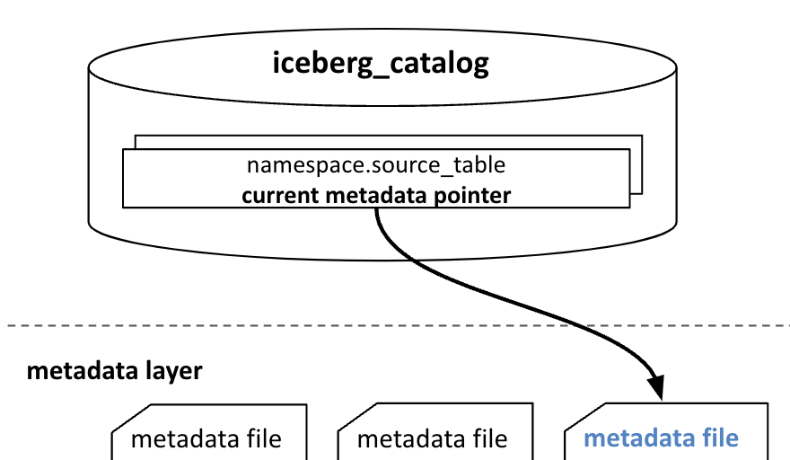
The first key component of Iceberg is the Catalog. A catalog manages tables grouped by namespaces and handles all operations such as creation, deletion, and modification of tables. To perform these tasks, a catalog contains a Current Metadata Pointer, which serves as an entry point by indicating the most recent metadata file of an Iceberg table when any operations are performed on it.
Additionally, a catalog enables monitoring the state of ongoing transactions on a table, ensuring a consistent view of the table – an essential requirement for ACID. However, transaction checks can only occur within the same type of catalog. If multiple types of catalogs are used for a single Iceberg table, the state of ongoing transactions cannot be verified across different types of catalogs, making it impossible to guarantee a consistent view. For example, if a table is committed through one type of catalog, other types may still show its previous state.
Next, let me introduce the type of catalogs. Compatible catalogs with Iceberg are generally classified into service catalogs and file-system catalogs.
Service catalogs, such as on-premise or cloud-managed services (e.g., AWS), maintain all references to Iceberg tables using a backup storage and ensure ACID through a locking mechanism. A notable example is Nessie, which focuses on version control similar to Git. Another service catalog, Hive Metastore, is advantageous for teams already familiar with Hive environments, which is why our team currently uses it. Additionally, AWS Glue, Snowflake, and JDBC are also available for Iceberg catalog.
Conversely, an example of a file-system catalog is the Hadoop catalog. It tracks the most recent version of tables using a version-hint.txt file in the file system. While service catalogs provide convenient functions (e.g., concurrency control) and specialized features for specific purposes(e.g. Nessie’s version control feature), file system catalog only provides basic storage capability, so this is generally not recommended for production services.
Metadata and Data Layer
The components within Iceberg’s metadata layer that I will introduce include the metadata file, manifest list, and manifest files. The metadata layer contains all necessary information except for the actual data and is essential for Iceberg’s core functionalities.
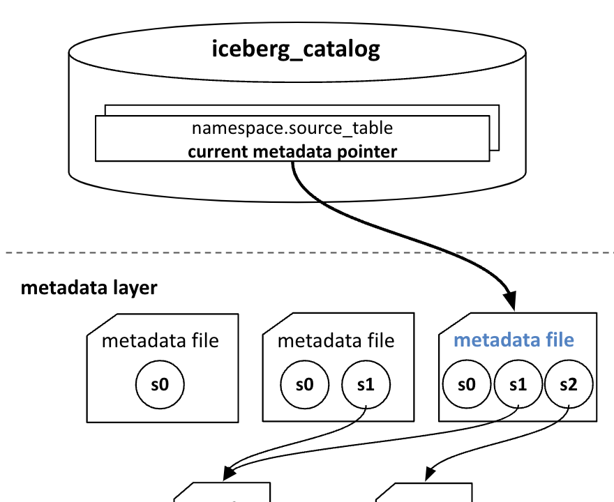
The first component in the metadata layer is the metadata file. As mentioned earlier, the catalog holds a current metadata pointer, which points to the most recent metadata file. A new metadata file is created every time a commit is successfully executed on an Iceberg table, and the current metadata pointer is updated to refer to this newly created metadata file. The commit is performed atomically, ensuring no loss of data in concurrent environments. This feature guarantees that the new metadata file is generated and replaced based on the previous version.
The metadata file contains basic information about the table as well as details about the snapshots being tracked. This basic information includes the table’s unique ID, applied settings, schema details, and storage paths for related files, and more. Additionally, it includes a sequence number indicating the relative age of the snapshot. The metadata file also holds statistical information such as record and file counts, as well as the storage paths for associated manifest lists. Iceberg uses this information to check the manifest list of a specific snapshot, read only the necessary files, and provide results in a table format when a user queries the state of the table at a specific time.
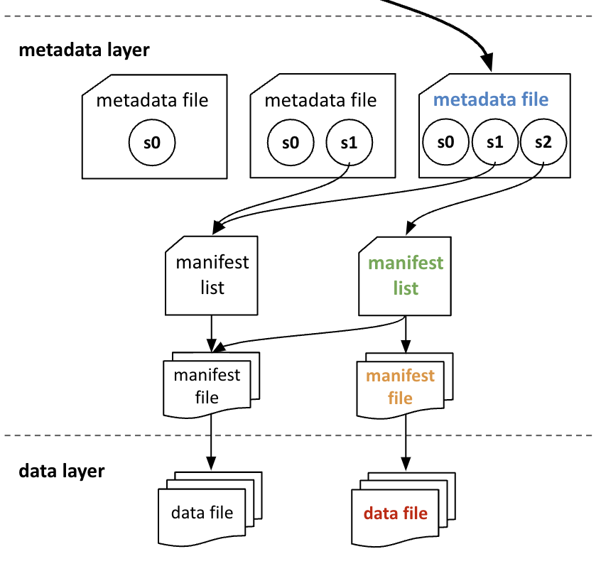
Next, I will discuss the manifest list within the metadata layer. A manifest list is a file containing information about a specific snapshot. In contrast to the snapshot, which represents the table’s state at a certain point in time, the manifest list is a physical file associated with that snapshot. It includes a list of all the manifest files created after a commit. Also, it contains data such as the type of manifest files, statistics like the number of added or deleted records, and partition information.
The final component in the metadata layer is the manifest file, which corresponds to data files and delete files. A manifest file holds type information about the files it references, such as data file, equality delete file, which holds deletion based on equality field columns, and position delete file, which includes deletion based on file path and position. Similar to the manifest list, it stores statistical information such as the minimum and maximum values and the number of null values for each column, along with the path of each manifest file. This information is utilized to identify only the specific manifest files needed for queries.
In the data layer, actual data and changes are stored in files. The data file contains all the data except for delete records. As for delete files, the equality delete file stores the values of equality field columns, while the position delete file stores file path and position information. The example below shows the information stored in both the data file and the two types of delete files. It’s important to note that the equality delete file includes the values of all equality field columns id which are present in the data file. The reasons for this will be explained in detail in the upcoming sections “Sink Operator ” and “Scan Planning”.
// data file
   id first_name last_name                email  phone_number job_title    salary  department_id  is_active
0  23   seungmin       lee seungmin@example.com 010-4321-9876  Employee  30000.00              1          1
1  24    Unknown   Unknown                 null          None      None      0.00             -1          0
2  25    gildong      hong  gildong@example.com 010-1234-5678  Employee  50000.00              1          1

// equality delete file
   id
0  23
1  24
2  25

// position delete file
                                                                                                                           file_path   pos
0   hdfs://hadoop-cluster/.../.../namespace/source_table/data/id_bucket=0/00000-0-6215b83a-023c-409e-8c6d-d9460bdf23a7-00009.parquet     1
< Example 1: Data file, equality delete file, and position delete file >
Key Configuration of Iceberg Table
Iceberg offers various configurations. Although I can’t cover all of them here, I will explain two key configurations that our team found important during testing and research, and which we are currently using. More details about other configurations and values we use can be found in the section “Iceberg Table Configuration”. Before discussing the two main settings, let me outline our team’s process for using Iceberg tables:
-
Create Iceberg tables using Flink
-
Load MySQL table data into the Iceberg table
-
Query Iceberg tables using Spark
Now, let’s dive into the key configurations of Iceberg tables.
The first configuration is the table’s write mode. The write mode can be individually set using the write.update.mode, write.delete.mode, and write.merge.mode options. The available values are COW (Copy-on-Write) and MOR (Merge-on-Read). This configuration determines how data is loaded and queried. For instance, setting it to COW mode updates existing files during data loading, immediately reflecting changes. This incurs a high cost in write operation but offers lower costs when querying the table since files already incorporate changes. Conversely, with MOR mode, actual data and changes (deletions) are stored in separate files. These files are merged during queries, leading to lower costs for write operation but higher costs during queries due to data merging. Therefore, it is crucial to clearly understand the usage environment of Iceberg tables and choose an appropriate setting based on when you wish to incur most of the cost.
The second configuration is about partitioning. Iceberg allows setting partitions on specific columns, storing data in physically separated paths for each partition. Supported partition transforms (types) include:
-
Bucket: Partitions are created by hashing the partition column’s value and performing a modulo operation with a user-set modulo value. Our team currently uses this one.
-
Identity: Differentiates between each partition based on unique values in a partition column.
-
Truncate: Trims the partition column’s value to a user-set integer length before performing an identity partition.
-
Hour, Day, Month, Year: Separates partitions based on time information in a partition column.
Regarding partitioning, two considerations need to be addressed. The first is that partitioning does more than just separating data physically for storage; it also significantly impacts Iceberg’s performance. In particular, if data is loaded using MOR mode and changes need to be incorporated during queries, setting partitions can greatly enhance performance. With partitions set, file comparison and merging are performed at the partition level, improving query efficiency. Additionally, compaction, one of Iceberg’s key maintenance features, is also performed per partition, allowing faster execution. More details will be discussed in the upcoming section “Scan Planning and Maintenance of Iceberg”. However, overly granular partitions can lead to the creation of many small files, negatively affecting performance. Hence, appropriately setting partitions is crucial.
The second consideration is that Iceberg does not allow multiple partitions on the same column. Some users might set multiple levels of partitions on time-related columns (e.g. /ts_column_year=.../ts_column_month=.../), complicating management and potentially degrading performance due to excessive granularity, as previously mentioned. Fortunately, the Iceberg community has taken action to prevent this (Improve partition spec builder · apache/iceberg · GitHub). Nonetheless, while it might be possible to do this using ALTER TABLE queries through Spark SQL or similar methods instead of the library-provided API, it is advised not to set multiple partitions on the same column to avoid errors during queries.
Preparing for Flink to Iceberg
Our team loads data into Iceberg tables using Flink. Therefore, we needed to configure not just Iceberg, but also Flink and some related systems.
In this section, I will share some of the specific configurations and brief code that we applied when loading data from MySQL tables into Iceberg tables on the Hadoop File System using Flink. Please note that these configurations are not definitive solutions; there may be more suitable configurations depending on the situation. To provide context, I will first clearly state our team’s mission and situation before explaining the configurations in detail.
-
Our team’s mission is to collect data needed for metrics. We map MySQL table column types to Iceberg table column types as long as it does not interfere with the metric calculations.
-
We use the Hadoop File System for object storage and the Hive Metastore as the catalog, as our team is already familiar with Hadoop and Hive environments.
-
To ensure idempotency during reprocessing, we load data in
UPSERTmode. -
Each Flink job synchronizes with only one MySQL table. Although the Flink CDC library allows retrieving from multiple tables in a single Flink job, Iceberg’s Flink Sink API does not support data loading into multiple tables.
Flink Configuration
First, let me share some of the configurations and values we set up in Flink. The first configuration relates to Hadoop authentication, and the second one is the Flink checkpoint interval configuration.
Starting with the Hadoop authentication settings, since our team uses the Hadoop File System as an object storage, it’s necessary to configure Hadoop authentication in Flink. We use a Hadoop File System installed in-house, and authentication via Kerberos is supported. So the following settings are added to Flink’s flink-conf.yaml file. If you are using Flink version 1.19 or later, the flink-conf.yaml file has been replaced by conf.yaml, so apply the same settings in the conf.yaml file.
hadoop.security.authentication: kerberos
security.kerberos.login.principal: seungmin-lee@HADOOP
security.kerberos.login.keytab: /../../seungmin-lee.keytab
security.kerberos.access.hadoopFileSystems: hdfs://hadoop-cluster
< Configuration 1: Hadoop kerberos in Flink configuration >
Next is the checkpoint interval in Flink. Checkpoints are state snapshots that Flink periodically stores and are used to recover flink jobs if they fail. Generally, it’s recommended to set shorter checkpoint intervals when there is no load in the flink job. However, there are considerations when loading data into Iceberg. With flink jobs, data committed to an Iceberg table occurs at each checkpoint interval, leading to the creation of new files. This means that more frequent checkpoints lead to the creation of more, smaller files. And the creation of many small files is a primary reason for increased query execution time, which will be explained in more detail in the section “Scan Planning”.
However, increasing the checkpoint interval is not advisable due to stability reasons. Additionally, when it comes to querying Iceberg tables, data can only be queried after it has been committed. So increasing the checkpoint interval also creates challenges for real-time operations. For example, if data is loaded at 3:30 PM and the commit occurs at 3:50 PM, then the data loaded at 3:30 PM is only available for querying after 3:50 PM. After some testing, our team decided that a 10-minute interval would be the optimal checkpoint interval, as it allows for stable checkpointing and doesn’t interfere with metric calculations.
Hive Configuration
One important configuration to consider in Hive is the hive.metastore.disallow.incompatible.col.type.changes option related to DDL. This option is applied globally on the Hive server and determines whether column type changes in DDL are allowed. Before explaining this further, it’s important to note that Flink CDC does not support DDL events when synchronizing MySQL tables with Iceberg tables. As shown in Code 1 , it processes MySQL changes based on event types but always checks the “before” or “after” keys. However, DDL-related messages lack these keys and instead contain information about the executed DDL. Consequently, as discussed in the first article Journey with Apache Flink & Flink CDC, when a DDL event occurs, we skip the DDL and subsequent events. We then execute the DDL separately on the Iceberg table using Spark SQL or Trino and re-integrate using the GTIDs of the DDL.
public void deserialize(SourceRecord record, Collector out) throws Exception {
    Envelope.Operation op = Envelope.operationFor(record);
    Struct value = (Struct) record.value();
    Schema valueSchema = record.valueSchema();
    // CREATE, SELECT
    if (op == Envelope.Operation.CREATE || op == Envelope.Operation.READ) {
        GenericRowData insert = extractAfterRow(value, valueSchema);
        validator.validate(insert, RowKind.INSERT);
        insert.setRowKind(RowKind.INSERT);
        emit(record, insert, out);
    // DELETE
    } else if (op == Envelope.Operation.DELETE) {
        GenericRowData delete = extractBeforeRow(value, valueSchema);
        validator.validate(delete, RowKind.DELETE);
        delete.setRowKind(RowKind.DELETE);
        emit(record, delete, out);
    // UPDATE
    } else {
        if (changelogMode == DebeziumChangelogMode.ALL) {
            GenericRowData before = extractBeforeRow(value, valueSchema);
            validator.validate(before, RowKind.UPDATE_BEFORE);
            before.setRowKind(RowKind.UPDATE_BEFORE);
            emit(record, before, out);
        }

        GenericRowData after = extractAfterRow(value, valueSchema);
        validator.validate(after, RowKind.UPDATE_AFTER);
        after.setRowKind(RowKind.UPDATE_AFTER);
        emit(record, after, out);
    }
}
< Code 1: Deserialize records in Flink CDC >
However, even when executing DDL with Spark SQL or Trino, the default option value of hive.metastore.disallow.incompatible.col.type.changes is true, which means that column type changes are not supported by default. Whether a DDL event causes a column type change can be understood by examining Iceberg’s metadata files. For example, if the type of the n-th column in the partition information within the metadata file changes after a DDL event, it is considered a type change. Reordering columns is also considered as a type change in metadata files and it is not allowed. If a table only has columns of the same type, changing the order might be successful. Without changing this setting, trying to alter a column type will produce Error Message 1 . Therefore, to allow type changes, you must set hive.metastore.disallow.incompatible.col.type.changes to false.
The following columns have types incompatible with the existing columns in their respective positions
< Error Message 1: DDL error >
Catalog and Namespace Configuration
In the catalog, you need to configure the table type, catalog type, and the path where files will be stored. The table type should always be set to iceberg, and since we use the Hive metastore, the catalog type is specified as hive. The WAREHOUSE_LOCATION configuration specifies the path where all data and metadata files for the tables will be stored. Therefore, it’s recommended to combine the namespace and table name to set separate paths for each table. Additionally, to use Hive as a catalog, you must add the Thrift URI of the Hive metastore to the uri configuration. However, in our case, the Hadoop and Hive settings are already included in the container image used by our Flink, so no additional configuration was necessary.
Finally, specifying a namespace is not mandatory. However, pre-defining the owner of the namespace and table can be helpful for future operations and permissions management. For these reasons, we added settings related to the owner of the namespace and table, as shown below.
import org.apache.iceberg.flink.CatalogLoader

hiveCatalogProps.put("type", "iceberg")
hiveCatalogProps.put("catalog-type", "hive")
hiveCatalogProps.put("warehouse", s"hdfs://hadoop-cluster/../../${namespace}/${table}")
val hivecatalog = CatalogLoader.hive("catalog_name", hadoopConf, hiveCatalogProps)

namespaceProps.put(HiveCatalog.HMS_TABLE_OWNER, "seungmin-lee")
namespaceProps.put(HiveCatalog.HMS_DB_OWNER, "seungmin-lee")
hiveCatalog.createNamespace(Namespace.of("namespace_name"), namespaceProps)
< Code 2: Configure and create catalog, namespace >
Iceberg Table Configuration
When configuring Iceberg tables, there are aspects that need to align not only with the specific environment or purpose but also our team policies. First, since our team loads data in UPSERT mode to ensure idempotency when re-running flink jobs, we set write.upsert.enabled to true. In addition, using UPSERT mode requires a format-version of 2 or higher. As of January 2025, format-version 3 is still in development and not officially adopted, so we are using version 2. We also enable engine.hive.enabled because we consider querying Iceberg tables using the internally provided Hive or Trino.
We use the default Parquet for file type and zstd for compression. The default compression codec was gzip until Iceberg version 1.4, but zstd showed better performance and improved GC (Garbage Collection) stability when queried through Trino. Hence, the default compression codec was changed to zstd in later Iceberg versions.
Moreover, we configure write.metadata.delete-after-commit.enabled to true so that metadata files are automatically deleted after a commit. Since we use the Hadoop File System as object storage, creating files smaller than the Hadoop Block Size can negatively impact on the I/O performance of Hadoop File System. Also, there’s no need to retain all past metadata files as the latest metadata file contains all previous snapshot information unless Expire Snapshots feature is used, which will be explained in the upcoming section. We use the default retention count of 100.
Next, I will discuss the commit and write-related settings, which are crucial for operational stability. To improve reliability in case of commit failures, we increased the retry limit from the default of four times to sixty times. However, we reduced the maximum time limit for commit retries from the default of 30 minutes to 5 minutes, setting a threshold of 60 retries based on count and 5 minutes based on time. The write settings also include an isolation level setting, which determines how strictly the order is managed when multiple operators delete or update data simultaneously. In our environment, valid write operators to the Iceberg table always exist singly except during the incremental snapshot stage in CDC process. Hence, although write operations do not overlap, we use serializable, the default and strictest concurrency restriction, as a precaution.
tableProperties.put(TableProperties.COMMIT_NUM_RETRIES, "60") // 4(default) -> 60
tableProperties.put(TableProperties.COMMIT_TOTAL_RETRY_TIME_MS, "300000") // 30m(default) -> 5m
tableProperties.put(TableProperties.DEFAULT_FILE_FORMAT, "parquet")
tableProperties.put(TableProperties.ENGINE_HIVE_ENABLED, "true")
tableProperties.put(TableProperties.FORMAT_VERSION, "2")
tableProperties.put(TableProperties.METADATA_DELETE_AFTER_COMMIT_ENABLED, "true")
tableProperties.put(TableProperties.PARQUET_COMPRESSION, "zstd")
tableProperties.put(TableProperties.UPSERT_ENABLED, "true")
< Code 3: Configure Iceberg table >
As mentioned in the section “Iceberg Table Configuration”, partitioning is a key feature to configure. We generally set bucket partitions for primary keys. If a composite key consists of multiple columns, we use the column with the highest cardinality. When determining the modulo value for the bucket partition, we tested values of 5, 10, 25, and 50. As previously noted, highly granular partitions can negatively affect query performance. Tests showed that when the modulo value was 50 or higher, query execution times increased using Spark. Concluding that less granularity is better, we settled on a final value of 5.
Finally, regarding write mode configuration, our team uses the default COW setting when creating tables with Iceberg’s Flink API. Although this setting can significantly affect performance depending on the environment or method, Flink’s logic for writing to Iceberg tables always operates in MOR mode. Additionally, since only Flink performs write operations and all read operations are carried out through Spark and Trino in our environment, this setting is insignificant, so we did not specify it.
Loading Process from Flink to Iceberg
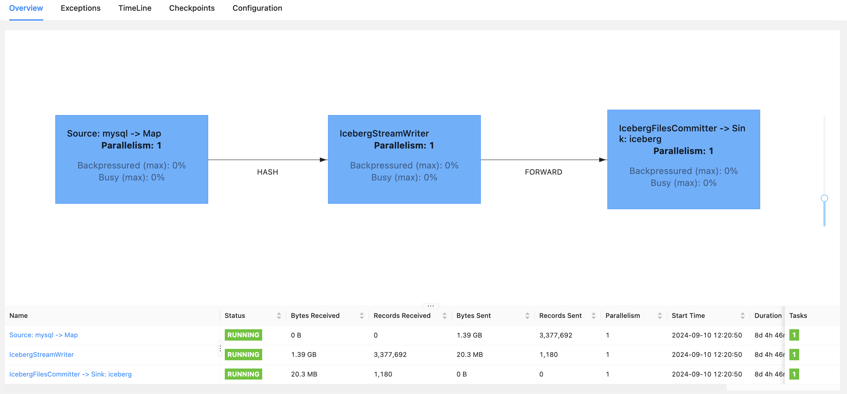
When loading data directly from Flink to Iceberg, RowData format is used instead of the ChangeEvent format utilized by Debezium through Kafka Connect. In this section, I will first explain the differences between RowData format and ChangeEvent format and discuss the advantages of using RowData format. Then explain how to dynamically create and use Flink Dynamic Tables and Iceberg tables when loading data from Flink to an Iceberg table. Finally, I will describe the operations of the three operators involved in loading data to an Iceberg table from Flink: Source, Sink, and Committer, along with the code examples.
Before diving into the detailed explanation, here is a brief overview of the roles of each operator:
-
Source: Retrieves data from MySQL table and generates messages in RowData format.
-
Sink: Loads data into the Iceberg table according to the event type of the message passed by the upstream operator.
-
Committer: Performs a commit to the Iceberg table when flink job executes checkpoints.
RowData type
CDC integration based on Debezium typically uses Kafka and Kafka Connect, sending messages in Debezium’s ChangeEvent format. ChangeEvent format is a JSON-type format that contains a variety of information, such as schema details, data before and after the query execution, source database information, and library details. An example of a ChangeEvent format message is shown in Example 2 below. As you can see from the example, because it holds such a variety of information, the message becomes heavy, negatively impacting message throughput.
If you want to lighten the message, you can utilize Schema Registry. However, this approach requires setting up and maintaining a server for the Schema Registry, which is a drawback. In a previous article Journey with Apache Flink & Flink CDC, we also discussed how data is loaded into the target MySQL table via Kafka and Kafka Connect, using the ChangeEvent format. The reason why direct data loading into the target MySQL table from Flink isn’t feasible is that Flink CDC mainly focused on source connectors. As of the time of writing, starting from Flink CDC version 3.0, it provides a pipeline connector that supports end-to-end data transfer from MySQL to Kafka.
{
  "schema": {
    "type": "struct",
    "fields": [
      {
        "type": "struct",
        "fields": [
          {
            "type": "int32",
            "optional": false,
            "field": "id"
          },
          {
            "type": "string",
            "optional": true,
            "default": "Unknown",
            "field": "first_name"
          },
          ...
        ],
        "optional": true,
        "name": "mysql_binlog_source.source_database.source_table.Value",
        "field": "before"
      },
      {
        "type": "struct",
        "fields": [
          {
            "type": "int32",
            "optional": false,
            "field": "id"
          },
          {
            "type": "string",
            "optional": true,
            "default": "Unknown",
            "field": "first_name"
          },
          ...
        ],
        "optional": true,
        "name": "mysql_binlog_source.source_database.source_table.Value",
        "field": "after"
      },
      ...
    ],
    "optional": false,
    "name": "mysql_binlog_source.source_database.source_table.Envelope"
  },
  "payload": {
    "before": null,
    "after": {
      "id": 23,
      "first_name": "seungmin",
      ...
    },
    "source": {
      "connector": "mysql",
      "name": "mysql_binlog_source",
      "db": "source_database",
      "table": "source_table",
      ...
    },
    "op": "r",
    "ts_ms": 1726664542015,
    "transaction": null
  }
}
< Example 2: ChangeEvent format >
However, Iceberg provides APIs for direct loading from Flink. This means that by using Flink CDC’s source connectors to retrieve MySQL data, you can directly load the data into an Iceberg table using Iceberg’s Flink Sink API. As a result, we don’t require Kafka anymore and need to use the ChangeEvent format; instead, Flink’s RowData format is used. When using the RowData format, table records and binary logs are categorized into three types within Flink. As shown in Example 3, the message types are +I(INSERT), +U(UPDATE_AFTER), and -D(DELETE).
+I(23,seungmin,lee,seungmin@example.com,010-4321-9876,Employee,30000.00,1,1)
+U(24,Unknown,Unknown,null,None,None,0.00,-1,0)
-D(25,gildong,hong,gildong@example.com,010-1234-5678,Employee,50000.00,1,1)
< Example 3: RowData format >
The reason CDC is possible with this simple format is that all the necessary information for CDC already exists in the flink job. This will be further explained in the section “Create Table Dynamically”. Additionally, since a flink job loads into one Iceberg table, there is no need to include information about the database or table in the message, unlike the ChangeEvent format.
The simplified message format improves message throughput, and as it eliminates the dependency on in-house Kafka, the upper limit on message throughput for users following in-house Kafka guidelines is also removed. As a result, we can increase message throughput as much as needed and complete the snapshot step of CDC integration more quickly, as long as we tune the database load well.
To share more about performance and execution time, when retrieving messages with Flink CDC and sending them to Kafka, the average throughput is about 5k msg/s per parallelism of 1 in a flink job (without Schema Registry). While increasing parallelism can boost throughput, in-house Kafka guidelines and limits on message throughput related to table size, preventing full utilization of Flink’s distributed processing capabilities during the incremental snapshot step of CDC integration.
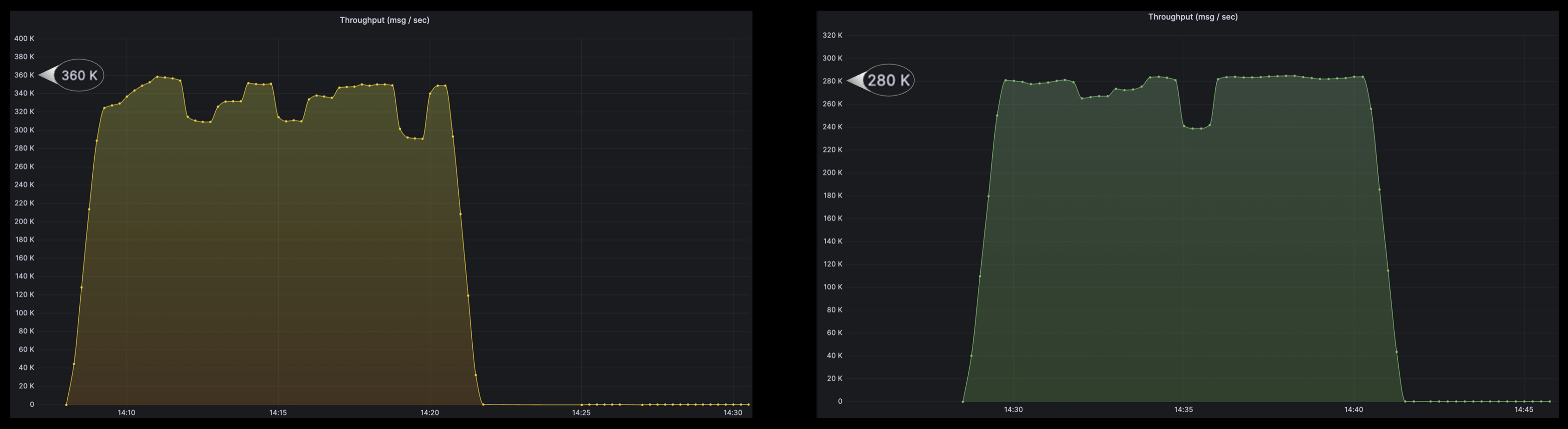
However, in a structure where data is loaded directly into Iceberg tables, the dependence on Kafka is removed, so we don’t need to consider in-house Kafka guidelines. Additionally, with the lighter message format, the throughput is approximately 15k msg/s per parallelism of 1 in a flink job. The only factor to consider is the database load. Performance limit tests conducted in collaboration with the in-house DBA team indicated that a maximum parallelism of up to 45 could be used. Assuming a parallelism of 40, the expected upper limit of message throughput is approximately 600k msg/s, far exceeding the limits present in in-house Kafka guidelines. Recent throughput for two flink jobs performing CDC integration on Iceberg tables, the peak message throughputs were 360k msg/s and 280k msg/s respectively, as shown in Figure 5 below. Both flink jobs had a parallelism of 20.
Create Table Dynamically
When running a flink job to load data into an Iceberg table, you need to dynamically create two tables: the first is a flink dynamic table, and the second is the Iceberg table. In this section, I will discuss how to dynamically generate and use the table schema necessary for creating these tables. I will also explain the reasons for creating the Iceberg table through flink job and describe how column types for tables defined in each system are mapped.
Flink dynamic table is a crucial feature that must be used when loading tables from flink into Iceberg. To load data into an Iceberg table from flink, you must use Flink’s Table API, with the dynamic table being the core of this process. Flink dynamic table determines the data type for each column value in a MySQL table. This is because it reads and converts each column’s value from the MySQL table to match the column types of the flink dynamic table.
For example, if a column in a MySQL table with an integer type is mapped to a column in the flink dynamic table with a string type, the integer values will be converted to string values. Typically, to create a flink dynamic table, you can specify the schema information required for table creation directly in the code, as shown in Code 4, or include it in a configuration file to be dynamically retrieved by a flink job. However, including table schema information in code or configuration files is not advisable for security reasons. Additionally, given that schemas may change unexpectedly, managing such information in files can be problematic from an operational perspective.
Similarly, as shown in Code 4, you can specify the necessary schema information in code or files to create Iceberg tables within a flink job. However, Iceberg tables can also be created using other methods, such as through separate engines like Spark or Trino. And generally, creating tables in advance is widely used. However, using another engine to create tables introduces dependencies on systems other than Flink, which adds additional considerations and complicates the overall CDC integration process.
// Flink Dynamic Table Schema
val flinkDynamicTableSchema = DataTypes.ROW(
  DataTypes.FIELD("id", DataTypes.BIGINT),
  DataTypes.FIELD("first_name", DataTypes.STRING),
  DataTypes.FIELD("last_name", DataTypes.STRING),
  DataTypes.FIELD("email", DataTypes.STRING),
  DataTypes.FIELD("phone_number", DataTypes.STRING),
  DataTypes.FIELD("job_title", DataTypes.STRING),
  DataTypes.FIELD("salary", DataTypes.STRING),
  DataTypes.FIELD("department_id", DataTypes.INT),
  DataTypes.FIELD("is_active", DataTypes.INT)
)

// Iceberg Table Schema
val icebergTableSchema = new Schema(
  Types.NestedField.required(1, "id", Types.LongType.get),
  Types.NestedField.optional(2, "first_name", Types.StringType.get),
  Types.NestedField.optional(3, "last_name", Types.StringType.get),
  Types.NestedField.optional(4, "email", Types.StringType.get),
  Types.NestedField.optional(5, "phone_number", Types.StringType.get),
  Types.NestedField.optional(6, "job_title", Types.StringType.get),
  Types.NestedField.optional(7, "salary", Types.StringType.get),
  Types.NestedField.optional(8, "department_id", Types.IntegerType.get),
  Types.NestedField.optional(9, "is_active", Types.IntegerType.get)
)
< Code 4: Statically create the table schemas >
There are also issues related to column types, as the column types in MySQL, flink dynamic table, and Iceberg table are defined separately for each system. This means that the column types in MySQL and flink dynamic table might not be compatible, nor might the column types in flink dynamic table and those in Iceberg table.
To address these issues, as shown in Example 4, we first execute the DESCRIBE TABLE command in the flink job on MySQL. We then use the results to dynamically generate the schemas needed to create both the flink dynamic table and the Iceberg table.
// MySQL Table Schema
+---------------+--------------+------+-----+---------+-------+
| Field         | Type         | Null | Key | Default | Extra |
+---------------+--------------+------+-----+---------+-------+
| id            | bigint       | NO   | PRI | NULL    |       |
| first_name    | varchar(50)  | NO   |     |         |       |
| last_name     | varchar(50)  | NO   |     |         |       |
| email         | varchar(100) | YES  |     | NULL    |       |
| phone_number  | varchar(20)  | NO   |     | NULL    |       |
| job_title     | varchar(50)  | YES  |     | NULL    |       |
| salary        | float        | NO   |     | 0.00    |       |
| department_id | int          | NO   |     | -1      |       |
| is_active     | tinyint(1)   | NO   |     | 1       |       |
+---------------+--------------+------+-----+---------+-------+

// Schema of Flink Dynamic Table based on MySQL Table Schema
ROW<
	`id` BIGINT,
	`first_name` STRING,
	`last_name` STRING,
	`email` STRING,
	`phone_number` STRING,
	`job_title` STRING,
	`salary` STRING,
	`department_id` INT,
	`is_active` INT
	>

// Schema of Iceberg Table based on MySQL Table Schema
table {
	1: id: required long (id) // used as equality field
	2: first_name: required string
	3: last_name: required string
	4: email: optional string
	5: phone_number: required string
	6: job_title: optional string
	7: salary: required string
	8: department_id: required int
	9: is_active: required int
}
< Example 4: Created schemas >
In the case of column type mapping, since our team’s primary goal is extracting daily metrics, having exactly the same column types is neither necessary nor always feasible. Instead, we establish mapping rules based on library code and tests to ensure that conversions between different column types are compatible and do not interfere with metrics extraction. The following Code 5 illustrates how conversions are handled in the library. By examining the convert function defined for each type, we can determine whether a conversion is allowed.
// Convert for Integer type
public Object convert(Object dbzObj, Schema schema) {
    if (dbzObj instanceof Integer) {
        return dbzObj;
    } else {
        return dbzObj instanceof Long ? ((Long)dbzObj).intValue() : Integer.parseInt(dbzObj.toString());
    }
}

// Convert for Long type
public Object convert(Object dbzObj, Schema schema) {
    if (dbzObj instanceof Integer) {
        return ((Integer)dbzObj).longValue();
    } else {
        return dbzObj instanceof Long ? dbzObj : Long.parseLong(dbzObj.toString());
    }
}
< Code 5: Type conversion in Flink CDC >
The column type mapping rules that our team currently uses are illustrated in Code 6 . To elaborate: first, integer types, float types, and some time-related types are set to the same type. For example, datetime type in MySQL is not supported in both flink dynamic tables and Iceberg tables, so it is mapped to the Timestamp type. Additionally, the bit length of MySQL’s bit type is first checked. If the bit length is 1, it is treated as boolean data and loaded as a String type. Otherwise, it is read as a VARBINARY type and loaded into Iceberg as a String type. The tinyint type is mapped to the int type because, although it’s often used to denote true or false with values 0 and 1, it sometimes stores values greater than 1. In such cases, converting to a String type would result in all values greater than 1 to be interpreted as true, leading to issues in metric extraction. Other types are all converted and loaded as String types.
import org.apache.flink.table.types.DataType
import org.apache.iceberg.types.Types

// Mapping rules for Flink Dynamic Table based on the result of DESC TABLE
case "int" => DataTypes.INT()
case "bigint" => DataTypes.BIGINT()
case "tinyint" => DataTypes.INT()
case "bit" if n > 1 => DataTypes.VARBINARY(n)
case "date" => DataTypes.DATE()
case "datetime" => DataTypes.TIMESTAMP(n)
case "timestamp" => DataTypes.TIMESTAMP(n)
case "float" => DataTypes.FLOAT()
case _ => DataTypes.STRING()

// Mapping rules for Iceberg Table based on the result of DESC TABLE
case "int" => Types.IntegerType.get
case "bigint" => Types.LongType.get
case "tinyint" => Types.IntegerType.get
case "datetime" => Types.TimestampType.withZone()
case "timestamp" => Types.TimestampType.withZone()
case "date" => Types.DateType.get
case "float" => Types.FloatType.get
case _ => Types.StringType.get
< Code 6: Type mapping rules >
Source Operator
Once the tables are dynamically created as described above, the source operator begins retrieving data from MySQL. During the incremental snapshot step, the source operator retrieves table data, and during the binlog stream step, it retrieves the binary log. It then converts the column values to match the schema of the flink dynamic table, and generates messages in RowData format.
Here is a brief overview of how the source operator works:
-
Connect to the database using the configured connection information.
-
Retrieve data from the MySQL table and binary logs.
-
Convert the retrieved values to match the column types of the flink dynamic table and generate messages in the RowData format.
-
Sends the generated messages to downstream operators.
To convert the read messages into the RowData format, you should use Flink CDC’s RowDataDebeziumDeserializeSchema function. If you prefer to convert to the existing JSON-type ChangeEvent format, use the JsonDebeziumDeserializationSchema. To use RowDataDebeziumDeserializeSchema, you need to convert the flink dynamic table schema of DataType type (shared in Code 4) to Flink’s TypeInformation[RowData] type. This conversion should proceed in the order of DataType, logicalType, and TypeInformation[RowData]. While you can convert them all at once using staticfromDataTypeToLegacyInfo function, this function is soon to be deprecated, so it’s recommended to follow the sequence mentioned earlier. For type conversions, you can use TypeConversions and InternalTypeInfo provided in Flink’s Table API. Below Code 7 shows an example of how to implement and use these type conversions. Updated February 2025: Please note that if you create directly RowData type and convert it to typeInfo, you can implement it more simply without creating a flink dynamic table.
MySqlSource.builder[A]()
  .hostname(...)
  .port(...)
  ...
  .deserializer(getRowDataDebeziumDeserializeSchema(flinkDynamicTableSchema))
  .build()

private def getRowDataDebeziumDeserializeSchema(flinkDynamicTableSchema: DataType): RowDataDebeziumDeserializeSchema = {
  val logicalType = TypeConversions.fromDataToLogicalType(flinkDynamicTableSchema)
  val typeInfo = InternalTypeInfo.of(logicalType).asInstanceOf[TypeInformation[RowData]]

  RowDataDebeziumDeserializeSchema.newBuilder
    .setPhysicalRowType(flinkDynamicTableSchema.getLogicalType.asInstanceOf[RowType])
    .setChangelogMode(DebeziumChangelogMode.UPSERT)
    .setResultTypeInfo(typeInfo)
    .build()
}
< Code 7: Deserialize with RowDataDebeziumDeserializeSchema >
Sink Operator
The sink operator loads data into the Iceberg table using RowData format messages sent from upstream operators. During this process, you can utilize the Flink Sink API provided by Iceberg library. Below, Code 8 is an example function for loading data into an Iceberg table. Since our team uses the UPSERT mode, we have added the necessary configuration for it. Additionally, when using UPSERT mode, you must always set equality field columns, which are used to determine if records are identical. Once the configuration is complete, as shown in the example, messages generated by the source operator are loaded into the Iceberg table through the sink operator.
import org.apache.iceberg.flink.sink.FlinkSink

FlinkSink.forRowData(rowDataFormatDataStream)
  .table(...)
  .tableLoader(...)
  .upsert(true)
  .equalityFieldColumns(pk)
  .append()
< Code 8: Sink to Iceberg using Iceberg sink API >
In the previous section, I explained that Iceberg manages data and metadata as files. Now, let me explain how messages are written to these files. Below, Code 9 shows a function used to load data into an Iceberg table, where the detailed behavior varies depending on the message type. Messages of types +I(INSERT) and +U(UPDATE_AFTER), which indicate data addition or update, follow the same logic. In the case of UPSERT mode, messages are also stored in delete files, ensuring that only the latest record is shown by removing previous record, when the table is queried. The criteria for how data is marked as deleted during table queries will be discussed in the below section “Scan Planning ”. Additionally, messages of type -D(DELETE) are always stored only in delete files.
public void write(RowData row) throws IOException {
	RowDataDeltaWriter writer = route(row);
	switch (row.getRowKind()) {
		case INSERT:
		case UPDATE_AFTER:
			if (upsert) {
				writer.deleteKey(keyProjection.wrap(row));
			}
			writer.write(row);
			break;
		case UPDATE_BEFORE:
			if (upsert) {
			  break;
			}
			writer.delete(row);
			break;
		case DELETE:
			if (upsert) {
				writer.deleteKey(keyProjection.wrap(row));
			} else {
				writer.delete(row);
			}
			break;
		default:
			throw new UnsupportedOperationException("Unknown row kind: " + row.getRowKind());
	}
}
< Code 9: Logic for writing data to Iceberg >
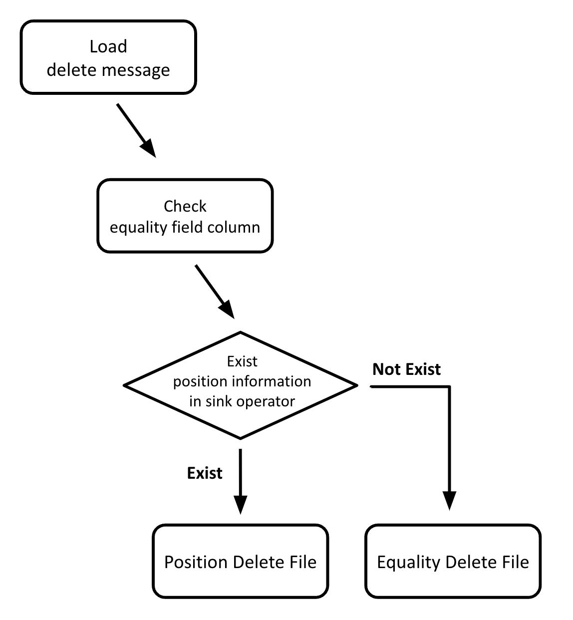
Now, let me explain delete files. I explained that there are two types: position delete file and equality delete file. The type of delete file used when data is deleted varies depending on how each engine is implemented. In Flink’s UPSERT mode, the logic for how delete messages are stored in delete files is depicted in Figure 6, and the delete file is determined and stored according to the flow below:
-
Check the equality field column value of the delete message.
-
Verify if a message with the same equality field column value exists in the memory of the sink operator. If the message has been ingested at least once during the same snapshot (referring to an Iceberg snapshot, not the snapshot phase) and by the same sink operator, it will exist in memory.
-
If the above condition is met, as there is a path of associated data file and position for the stored message, it is stored in a position delete file.
-
Otherwise, it is stored in an equality delete file.
Committer Operator
The committer operator plays a separate role from the flow of retrieving and loading data, committing to the Iceberg table according to the flink job’s checkpoint interval. Unlike the previous two operators, there is nothing the user needs to implement. As shown in Code 10, when the user configures the pipeline from the source operator to the sink operator, the library automatically adds a committer operator at the end of the user-defined pipeline.
private  DataStreamSink chainIcebergOperators() {

    ...
	// distributeStream = use-defined pipeline
	SingleOutputStreamOperator writerStream = appendWriter(distributeStream, flinkRowType, equalityFieldIds);

	// append committer operator at the end of pipeline
	SingleOutputStreamOperator committerStream = appendCommitter(writerStream);

	...
}
< Code 10: Add committer operator to user-defined pipeline >
The result of the commit is the creation of a snapshot, and if there are no incoming messages, an empty commit is performed, resulting in no changes. The related setting flink.max-continuous-empty-commits exists and the default value is 10. If 10 consecutive empty commits occur, a snapshot is created even if there are no changes. Below Figure 7 illustrates a snapshot creation example due to empty commits. With a flink job which has a checkpoint interval of 10 minutes, commits to the Iceberg table are performed every 10 minutes, and a new snapshot is created after 10 consecutive empty commits. These 10 consecutive empty commits equate to a time span of 1 hour and 40 minutes (10 minutes * 10 times), and as shown by the metadata file and manifest list creation timestamps in Figure 7, new files are generated every 1 hour and 40 minutes, at 11:14 am, 12:54 pm, and 1:34 pm.

Deep Dive into Metadata Over Time
In this section, I will examine the metadata file, manifest list, and manifest file of Iceberg tables with real examples. To better illustrate the actual operation process, I will explain the files created at each stage, the information each file contains, and how this information is utilized in the following order.
-
At the point of Iceberg table creation (at the time of the first metadata file creation)
-
First snapshot
-
Second snapshot
At the Point of Table Creation
When an Iceberg table is created, it takes the form shown in Figure 8 , and the first metadata file, as shown in Example 5, is generated.
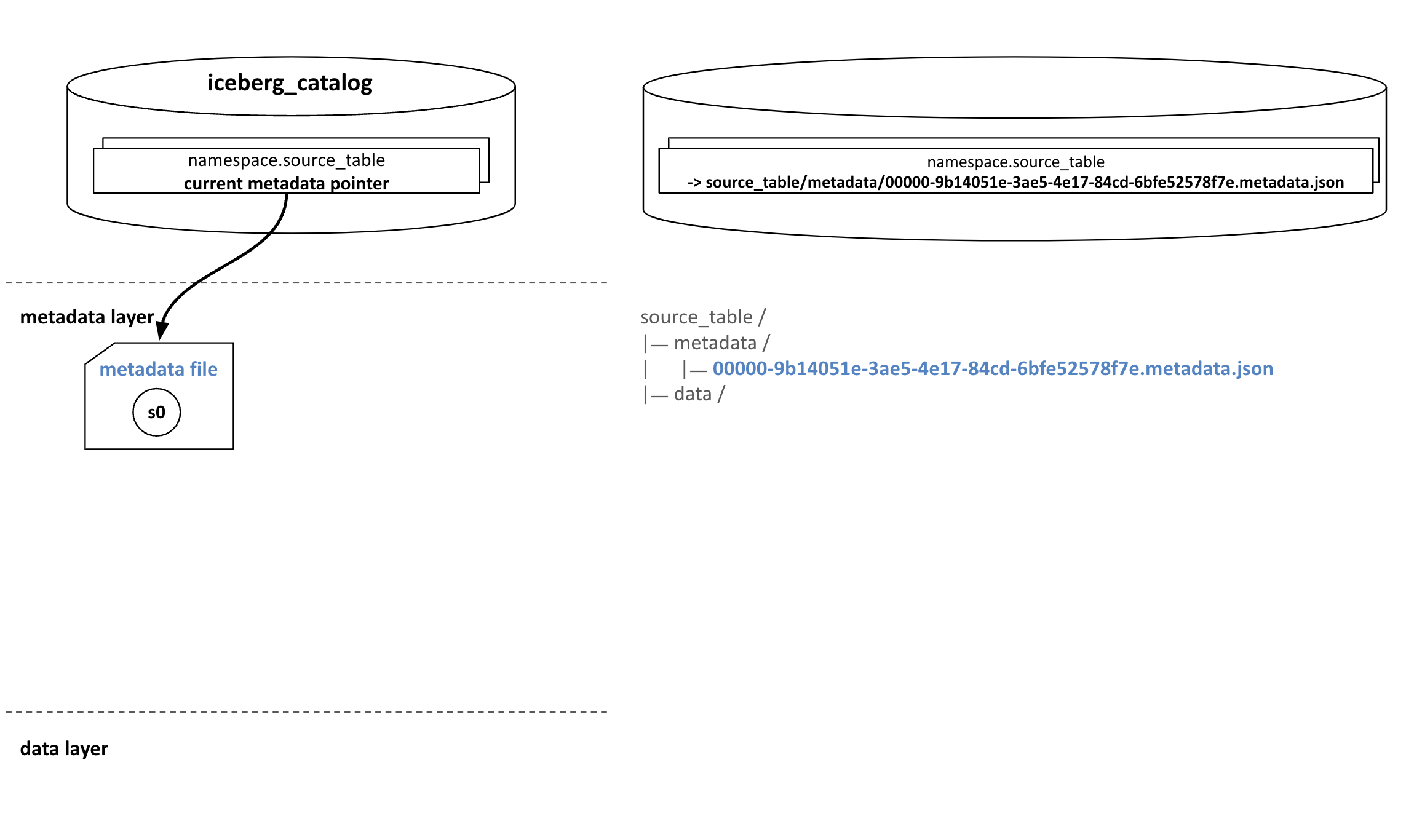
The metadata file stores information such as the unique ID of the created table, file storage locations, schema, and partition information. The schema and partition information are stored in list form to preserve the entire history of changes. Since Example 5 represents the state immediately after table creation, there is only one entry for each. Also, the initially assigned schema ID (schema-id) and spec ID (spec-id) are both set to 0.
You can also verify the table settings explained in the section “Iceberg Table Configuration ”. Specifically, you can see Hive-related settings, commit retry settings, and that it is configured in UPSERT mode. However, the current snapshot ID (current-snapshot-id) is set to -1 because no data has been loaded nor have any commits been made to create a snapshot. For the same reason, the snapshot-related information and metadata log information contain empty lists.
{
  "format-version" : 2,
  "table-uuid" : "884766bb-9cab-4298-829e-a096689d9ddc",
  "location" : "hdfs://hadoop-cluster/.../namespace/source_table",
  "last-sequence-number" : 0,
  "last-updated-ms" : 1723879432267,
  "last-column-id" : 9,
  "current-schema-id" : 0,
  "schemas" : [ {
    "type" : "struct",
    "schema-id" : 0,
    "identifier-field-ids" : [ 1 ],
    "fields" : [ {
      "id" : 1,
      "name" : "id",
      "required" : true,
      "type" : "int"
    },
    ... // skip
    {
      "id" : 9,
      "name" : "is_active",
      "required" : true,
      "type" : "int"
    } ]
  } ],
  "default-spec-id" : 0,
  "partition-specs" : [ {
    "spec-id" : 0,
    "fields" : [ {
      "name" : "id_bucket",
      "transform" : "bucket[5]",
      "source-id" : 1,
      "field-id" : 1000
    } ]
  } ],
  "last-partition-id" : 1000,
  "default-sort-order-id" : 0,
  "sort-orders" : [ {
    "order-id" : 0,
    "fields" : [ ]
  } ],
  "properties" : {
    "engine.hive.enabled" : "true",
    "commit.retry.total-timeout-ms" : "300000",
    "write.format.default" : "parquet",
    "write.parquet.compression-codec" : "zstd",
    "write.upsert.enabled" : "true",
    "write.metadata.delete-after-commit.enabled" : "true",
    "commit.retry.num-retries" : "60"
  },
  "current-snapshot-id" : -1,
  "refs" : { },
  "snapshots" : [ ],
  "statistics" : [ ],
  "partition-statistics" : [ ],
  "snapshot-log" : [ ],
  "metadata-log" : [ ]
}
< Example 5: Initial metadata file >
First Snapshot: Metadata File
When the first snapshot is created, new metadata files, manifest lists, manifest files, and data files are generated, as shown in Figure 9. The current metadata pointer is then updated to point to the newly created metadata file.
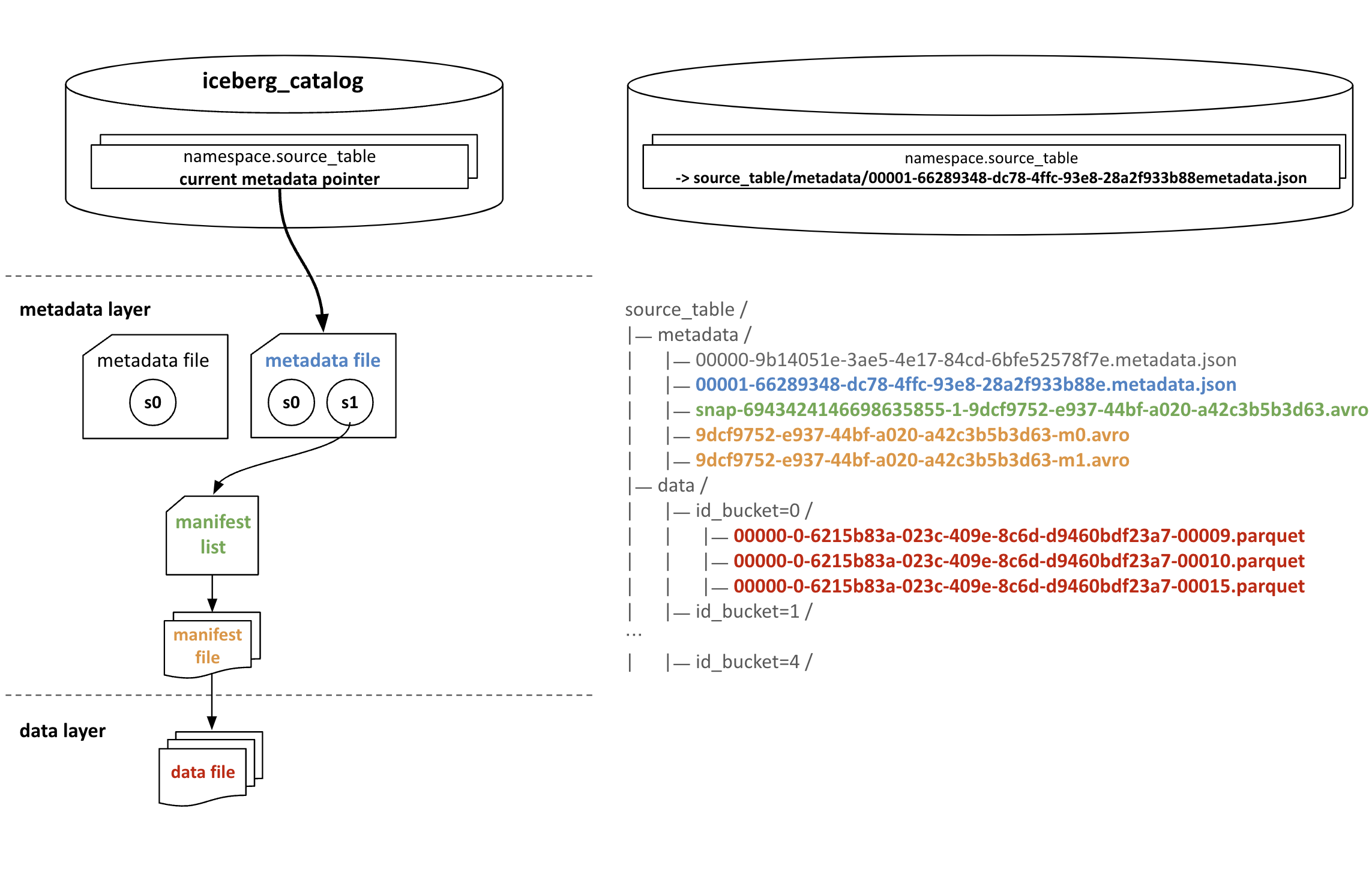
Example 6 below illustrates a newly created metadata file. A snapshot ID has been added, and since this is the first snapshot created, the sequence number that indicates the relative age of snapshots is set to 1. Additionally, there is a newly created snapshot summary information snapshots.summary in the snapshot-related information. The summary includes the number of records added and deleted, the number of files added and deleted, and the total number of files.
{
  "format-version" : 2,
  "table-uuid" : "884766bb-9cab-4298-829e-a096689d9ddc",
  "location" : "hdfs://hadoop-cluster/.../namespace/source_table",
  "last-sequence-number" : 1,
  "last-updated-ms" : 1723879779668,
  ... // skip
  "current-snapshot-id" : 6943424146698635855,
  "refs" : {
    "main" : {
      "snapshot-id" : 6943424146698635855,
      "type" : "branch"
    }
  },
  "snapshots" : [ {
    "sequence-number" : 1,
    "snapshot-id" : 6943424146698635855,
    "timestamp-ms" : 1723879779668,
    "summary" : {
      "operation" : "overwrite",
      "flink.operator-id" : "e883208d19e3c34f8aaf2a3168a63337",
      "flink.job-id" : "a40a5d923f750731620feafd9bf8930d",
      "flink.max-committed-checkpoint-id" : "1",
      "added-data-files" : "5",
      "added-equality-delete-files" : "5",
      "added-position-delete-files" : "5",
      "added-delete-files" : "10",
      "added-records" : "6971",
      "added-files-size" : "49492",
      "added-position-deletes" : "346",
      "added-equality-deletes" : "6625",
      "changed-partition-count" : "5",
      "total-records" : "6971",
      "total-files-size" : "49492",
      "total-data-files" : "5",
      "total-delete-files" : "10",
      "total-position-deletes" : "346",
      "total-equality-deletes" : "6625"
    },
    "manifest-list" : "hdfs://hadoop-cluster/../namespace/source_table/metadata/snap-6943424146698635855-1-9dcf9752-e937-44bf-a020-a42c3b5b3d63.avro",
    "schema-id" : 0
  } ],
  "statistics" : [ ],
  "partition-statistics" : [ ],
  "snapshot-log" : [ {
    "timestamp-ms" : 1723879779668,
    "snapshot-id" : 6943424146698635855
  } ],
  "metadata-log" : [ {
    "timestamp-ms" : 1723879432267,
    "metadata-file" : "hdfs://hadoop-cluster/../namespace/source_table/metadata/00000-9b14051e-3ae5-4e17-84cd-6bfe52578f7e.metadata.json"
  } ]
}
< Example 6: Metadata file generated from the first snapshot >
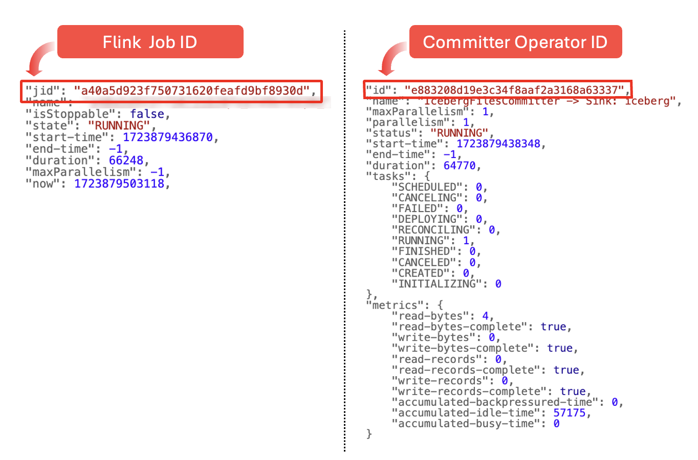
The summary information also contains details about the engine that performed the commit and created the snapshot. Since we are using Apache Flink, Flink-related information is included. To verify that this matches the actual flink job information, when querying the flink job ID via a REST API, it is retrieved as shown in Figure 10 , with the ID a40a5d923f750731620feafd9bf8930d. Comparing this value with the flink.job-id in Example 6 confirms they are identical. Additionally, the flink.operator-id includes the committer operator ID, which is also verified to be e883208d19e3c34f8aaf2a3168a63337 through a REST API, showing that both values are the same.
Information about snapshots created using engines other than Flink can also be identified through the summary information. Example 7 shows a snapshot created by performing a specific operation on the table using Apache Spark, along with a portion of the generated metadata file. While the previous information contains the Flink information, the summary information for this example contains the Spark application ID in spark.app_id.
{
  ..
  "snapshots" : [
  ...
  {
    "sequence-number" : 78,
    ...
    "summary" : {
      "operation" : "overwrite",
      "flink.operator-id" : "fbb4ef531e002f8fb3a2052db255adf5",
      "flink.job-id" : "fe781e5fbddd17d43e2290453dda4aa7",
      "flink.max-committed-checkpoint-id" : "1014",
      "added-data-files" : "5",
      "added-equality-delete-files" : "5",
      "added-position-delete-files" : "3",
      "added-delete-files" : "8",
      "added-records" : "271",
      "added-files-size" : "92717",
      "added-position-deletes" : "5",
      "added-equality-deletes" : "287",
      "changed-partition-count" : "5",
      "total-records" : "3420319",
      "total-files-size" : "330131861",
      "total-data-files" : "4601",
      "total-delete-files" : "5575",
      "total-position-deletes" : "1599",
      "total-equality-deletes" : "3422410"
    },
    "manifest-list" : "hdfs://hadoop-cluster/../namespace/source_table/metadata/snap-4930217877644357147-1-5f476623-f2ec-42b0-92d8-bef7dd5cd72d.avro",
    "schema-id" : 0
  },
  {
    "sequence-number" : 79,
    ...
    "summary" : {
      "operation" : "overwrite",
      "spark.app.id" : "application_1727068550645_39886",
      "added-data-files" : "989",
      "deleted-data-files" : "4601",
      "removed-equality-delete-files" : "4629",
      "removed-position-delete-files" : "938",
      "removed-delete-files" : "5567",
      "added-records" : "2966565",
      "deleted-records" : "3420319",
      "added-files-size" : "119275096",
      "removed-files-size" : "330120927",
      "removed-position-deletes" : "1594",
      "removed-equality-deletes" : "3422123",
      "changed-partition-count" : "5",
      "total-records" : "2966565",
      "total-files-size" : "119286030",
      "total-data-files" : "989",
      "total-delete-files" : "8",
      "total-position-deletes" : "5",
      "total-equality-deletes" : "287"
    },
    "manifest-list" : "hdfs://hadoop-cluster/../namespace/source_table/metadata/snap-8098152503420040164-1-db2d1c42-cd99-40cf-aea9-d322ace8bd62.avro",
    "schema-id" : 0
  } ]
  ...
}
< Example 7: Summary in metadata file created using Apache Spark >
First Snapshot: Manifest List
Now, let’s look at the manifest lists corresponding to the created snapshots. Example 8 is an example of a generated manifest list, enumerating information for two manifest files. If it was the manifest list for the second snapshot, information for a total of four manifest files would be listed, and all manifest files would accumulate until the Expire Snapshots feature discussed later is executed. Each manifest file information includes a content field, which indicates whether the manifest file corresponds to data files or delete files. A value of 0 indicates data files, and 1 indicates delete files. Therefore, the first manifest file 9dcf9752-e937-44bf-a020-a42c3b5b3d63-m0.avro corresponds to data files, while the second manifest file 9dcf9752-e937-44bf-a020-a42c3b5b3d63-m1.avro corresponds to delete files.
Additionally, the manifest files store sequence numbers, partition information, and statistical information such as the number of files or records added and deleted. Among these, the sequence number is used to determine whether delete files are reflected in data files during table queries, with the detailed process explained in the below section “Scan Planning ”. The partition information stores the upper_bound and lower_bound of partition columns. Since a modulo value of 5 is used for bucket partitioning, the upper and lower bounds are set to 4 and 0, respectively, and the actual stored values are base64-encoded, representing 0 and 4.
[{
  "manifest_path" : "hdfs://hadoop-cluster/.../namespace/source_table/metadata/9dcf9752-e937-44bf-a020-a42c3b5b3d63-m0.avro",
  "manifest_length" : 7668,
  "partition_spec_id" : 0,
  "content" : 0, // indicate data file
  "sequence_number" : 1,
  "min_sequence_number" : 1,
  "added_snapshot_id" : 6943424146698635855,
  "added_files_count" : 5,
  "existing_files_count" : 0,
  "deleted_files_count" : 0,
  "added_rows_count" : 6971,
  "existing_rows_count" : 0,
  "deleted_rows_count" : 0,
  "partitions" : [ {
    "contains_null" : false,
    "contains_nan" : false,
    "lower_bound" : "AAAAAA==", // Encoded in Base64. "00 00 00 00" means 0.
    "upper_bound" : "BAAAAA=="  // Encoded in Base64. "04 00 00 00" means 4.
  } ]
},
{
  "manifest_path" : "hdfs://hadoop-cluster/.../namespace/source_table/metadata/9dcf9752-e937-44bf-a020-a42c3b5b3d63-m1.avro",
  "manifest_length" : 7616,
  "partition_spec_id" : 0,
  "content" : 1, // indicate delete file
  "sequence_number" : 1,
  "min_sequence_number" : 1,
  "added_snapshot_id" : 6943424146698635855,
  "added_files_count" : 10,
  "existing_files_count" : 0,
  "deleted_files_count" : 0,
  "added_rows_count" : 6971,
  "existing_rows_count" : 0,
  "deleted_rows_count" : 0,
  "partitions" : [ {
    "contains_null" : false,
    "contains_nan" : false,
    "lower_bound" : "AAAAAA==",
    "upper_bound" : "BAAAAA=="
  } ]
}]
< Example 8: Manifest list generated from the first snapshot >
First Snapshot: Manifest File
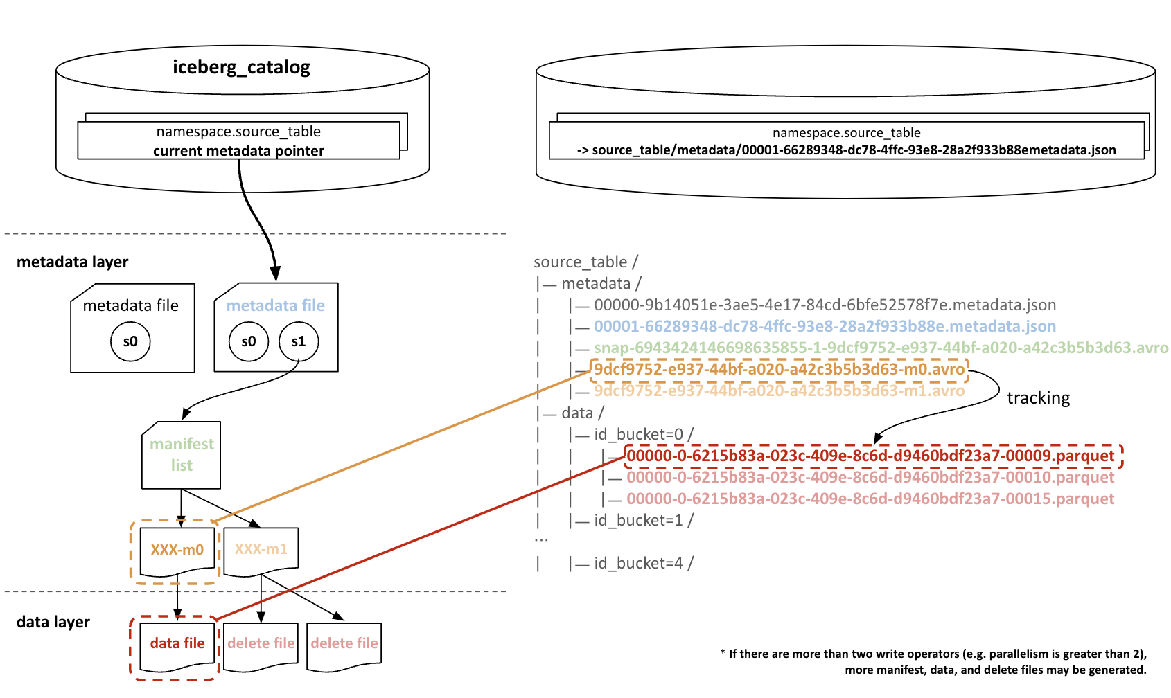
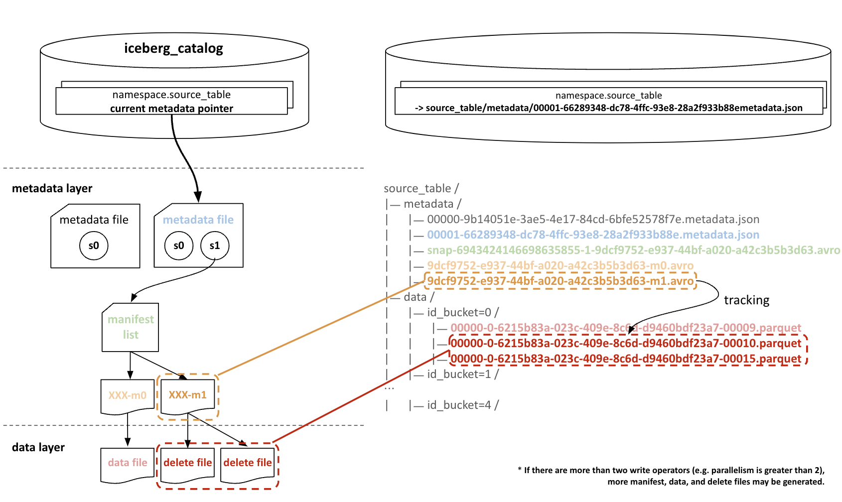
Finally, let’s verify the manifest files present in the manifest list. First, as mentioned earlier, each manifest file corresponds to data files or delete files. As shown in Figures 11 and 12 , the file 9dcf9752-e937-44bf-a020-a42c3b5b3d63-m0.avro corresponds to data files, including 00000-0-6215b83a-023c-409e-8c6d-d9460bdf23a7-00009.parquet, while 9dcf9752-e937-44bf-a020-a42c3b5b3d63-m1.avro corresponds to delete files, including 00000-0-6215b83a-023c-409e-8c6d-d9460bdf23a7-00010.parquet and 00000-0-6215b83a-023c-409e-8c6d-d9460bdf23a7-00015.parquet. The figures only show one partition to keep the image concise, but each manifest file actually corresponds to all data files and delete files, as explained.
By examining Example 9 , which is an example of a manifest file corresponding to data files, you can see that it lists information for all data files created in that snapshot. In Example 9 , since a modulo value of 5 is used for bucket partitioning, there are a total of five data files. Looking at the information within each data file, the first item is the status, indicating whether the manifest file represents an existing file (0: EXISTING), a newly added file (1: ADDED), or a deleted file (2: DELETED). In this example, all are newly added files with a value of 1. Additionally, each data file includes the snapshot ID and sequence number in which it was created. A sequence number null means it inherits the sequence number from the corresponding manifest file.
Looking further into the details in data_file, there is statistical information for each column and information about which bucket partition each data file belongs to (e.g., id_bucket=0). This information, like a sequence number, determines whether delete files should be applied to data files. For instance, partition information is used to check if the data files and delete files belong to the same partition, and statistical information is used to verify if the range of equality field columns in delete files overlaps with those in data files. The detailed process of merging files using this provided information will be thoroughly explained in the section “Scan Planning”.
[{
  "status" : 1,
  "snapshot_id" : 6943424146698635855,
  "sequence_number" : null,
  "file_sequence_number" : null,
  "data_file" : {
    "content" : 0,
    "file_path" : "hdfs://hadoop-cluster/.../namespace/source_table/data/id_bucket=0/00000-0-6215b83a-023c-409e-8c6d-d9460bdf23a7-00009.parquet",
    "file_format" : "PARQUET",
    "partition" : {
      "id_bucket" : 0
    },
    "record_count" : 1632,
    "file_size_in_bytes" : 6223,
    "column_sizes" : [...],
    "value_counts" : [...],
    "null_value_counts" : [...],
    "nan_value_counts" : [ ],
    "lower_bounds" :  [...],
    "upper_bounds" :  [...],
    "key_metadata" : null,
    "split_offsets" : [ 4 ],
    "equality_ids" : null,
    "sort_order_id" : 0
  }
},
{
  "status" : 1,
  "snapshot_id" : 6943424146698635855,
  "sequence_number" : null,
  "file_sequence_number" : null,
  "data_file" : {
    "content" : 0,
    "file_path" : "hdfs://hadoop-cluster/.../namespace/source_table/data/id_bucket=1/00000-0-6215b83a-023c-409e-8c6d-d9460bdf23a7-00005.parquet",
    "file_format" : "PARQUET",
    "partition" : {
      "id_bucket" : 1
    }
    ... // skip
},
{
  "status" : 1,
  "snapshot_id" : 6943424146698635855,
  "sequence_number" : null,
  "file_sequence_number" : null,
  "data_file" : {
    "content" : 0,
    "file_path" : "hdfs://hadoop-cluster/.../namespace/source_table/data/id_bucket=2/00000-0-6215b83a-023c-409e-8c6d-d9460bdf23a7-00001.parquet",
    "file_format" : "PARQUET",
    "partition" : {
      "id_bucket" : 2
    }
    ... // skip
},
{
  "status" : 1,
  "snapshot_id" : 6943424146698635855,
  "sequence_number" : null,
  "file_sequence_number" : null,
  "data_file" : {
    "content" : 0,
    "file_path" : "hdfs://hadoop-cluster/.../namespace/source_table/data/id_bucket=3/00000-0-6215b83a-023c-409e-8c6d-d9460bdf23a7-00007.parquet",
    "file_format" : "PARQUET",
    "partition" : {
      "id_bucket" : 3
    }
    ... // skip
  }
},
{
  "status" : 1,
  "snapshot_id" : 6943424146698635855,
  "sequence_number" : null,
  "file_sequence_number" : null,
  "data_file" : {
    "content" : 0,
    "file_path" : "hdfs://hadoop-cluster/.../namespace/source_table/data/id_bucket=4/00000-0-6215b83a-023c-409e-8c6d-d9460bdf23a7-00003.parquet",
    "file_format" : "PARQUET",
    "partition" : {
      "id_bucket" : 4
    }
    ... // skip
  }
}]
< Example 9: Manifest file corresponding to the data files >
The manifest file corresponding to delete files is shown in Example 10, which contains information for a total of ten delete files. Since two types of delete files are created for each of the five bucket partitions, there are ten delete files in total. However, this number may vary depending on how the engine implements the logic for writing delete files, so it should be understood that up to ten delete files can be created, not necessarily always ten. The information stored is almost identical to that of manifest files corresponding to data files, including status information, snapshot ID, sequence number, file path, partition information, and statistical information for each column.
The difference between manifest files corresponding to delete files and those for data files lies in the content field, which contains values of 1 or 2 for delete files. Here, 1 signifies position delete files, and 2 signifies equality delete files. Additionally, equality delete files list the numbers of equality field columns in equality_ids. In this example, the values 1 and 2 are present, indicating that the first and second columns are used as equality field columns.
[{
  "status": 1,
  "snapshot_id": 6943424146698635855,
  "sequence_number": null,
  "file_sequence_number": null,
  "data_file": {
    "content": 2, // 2 = equality delete file
    "file_path": "hdfs://hadoop-cluster/.../namespace/source_table/data/id_bucket=0/00000-0-6215b83a-023c-409e-8c6d-d9460bdf23a7-00010.parquet",
    "file_format": "PARQUET",
    "partition": {
      "id_bucket": 0
    },
    "record_count": 1555,
    "file_size_in_bytes": 1983,
    "column_sizes": [...],
    "value_counts": [...],
    "null_value_counts": [...],
    "nan_value_counts": [],
    "lower_bounds": [...],
    "upper_bounds": [...],
    "key_metadata": null,
    "split_offsets": [ 4 ],
    "equality_ids": [ 1, 2 ],
    "sort_order_id": 0
  }
},
{
  "status": 1,
  "snapshot_id": 6943424146698635855,
  "sequence_number": null,
  "file_sequence_number": null,
  "data_file": {
    "content": 1,
    "file_path": "hdfs://hadoop-cluster/.../namespace/source_table/data/id_bucket=0/00000-0-6215b83a-023c-409e-8c6d-d9460bdf23a7-00015.parquet",
    "file_format": "PARQUET",
    "partition": {
      "id_bucket": 0
    },
    "record_count": 77,
    "file_size_in_bytes": 1997,
    "column_sizes": [
      {
        "key": 2147483546, // means file_path column of position delete file
        "value": 219
      },
      {
        "key": 2147483545, // means pos column of position delete file
        "value": 154
      }
    ],
    "value_counts": null,
    "null_value_counts": null,
    "nan_value_counts": null,
    "lower_bounds": [...],
    "upper_bounds": [...],
    "key_metadata": null,
    "split_offsets": [ 4 ],
    "equality_ids": null,
    "sort_order_id": null
  }
},
{
  "status": 1,
  "snapshot_id": 6943424146698635855,
  "sequence_number": null,
  "file_sequence_number": null,
  "data_file": {
    "content": 2,
    "file_path": "hdfs://hadoop-cluster/.../namespace/source_table/data/id_bucket=1/00000-0-6215b83a-023c-409e-8c6d-d9460bdf23a7-00006.parquet",
    "file_format": "PARQUET",
    "partition": {
      "id_bucket": 1
    },
    ... // skip
  }
},
{
  "status": 1,
  "snapshot_id": 6943424146698635855,
  "sequence_number": null,
  "file_sequence_number": null,
  "data_file": {
    "content": 1,
    "file_path": "hdfs://hadoop-cluster/.../namespace/source_table/data/id_bucket=1/00000-0-6215b83a-023c-409e-8c6d-d9460bdf23a7-00011.parquet",
    "file_format": "PARQUET",
    "partition": {
      "id_bucket": 1
    },
    ... // skip
  }
},
{
  "status": 1,
  "snapshot_id": 6943424146698635855,
  "sequence_number": null,
  "file_sequence_number": null,
  "data_file": {
    "content": 2,
    "file_path": "hdfs://hadoop-cluster/.../namespace/source_table/data/id_bucket=1/00000-0-6215b83a-023c-409e-8c6d-d9460bdf23a7-00006.parquet",
    "file_format": "PARQUET",
    "partition": {
      "id_bucket": 2
    },
	... // skip
  }
},
{
  "status": 1,
  "snapshot_id": 6943424146698635855,
  "sequence_number": null,
  "file_sequence_number": null,
  "data_file": {
    "content": 1,
    "file_path": "hdfs://hadoop-cluster/.../namespace/source_table/data/id_bucket=1/00000-0-6215b83a-023c-409e-8c6d-d9460bdf23a7-00011.parquet",
    "file_format": "PARQUET",
    "partition": {
      "id_bucket": 2
    },
	... // skip
  }
},
{
  "status": 1,
  "snapshot_id": 6943424146698635855,
  "sequence_number": null,
  "file_sequence_number": null,
  "data_file": {
    "content": 2,
    "file_path": "hdfs://hadoop-cluster/.../namespace/source_table/data/id_bucket=2/00000-0-6215b83a-023c-409e-8c6d-d9460bdf23a7-00002.parquet",
    "file_format": "PARQUET",
    "partition": {
      "id_bucket": 3
    },
	... // skip
  }
},
{
  "status": 1,
  "snapshot_id": 6943424146698635855,
  "sequence_number": null,
  "file_sequence_number": null,
  "data_file": {
    "content": 1,
    "file_path": "hdfs://hadoop-cluster/.../namespace/source_table/data/id_bucket=3/00000-0-6215b83a-023c-409e-8c6d-d9460bdf23a7-00013.parquet",
    "file_format": "PARQUET",
    "partition": {
      "id_bucket": 3
    },
	... // skip
  }
},
{
  "status": 1,
  "snapshot_id": 6943424146698635855,
  "sequence_number": null,
  "file_sequence_number": null,
  "data_file": {
    "content": 2,
    "file_path": "hdfs://hadoop-cluster/.../namespace/source_table/data/id_bucket=4/00000-0-6215b83a-023c-409e-8c6d-d9460bdf23a7-00004.parquet",
    "file_format": "PARQUET",
    "partition": {
      "id_bucket": 4
    },
	... // skip
  }
},
{
  "status": 1,
  "snapshot_id": 6943424146698635855,
  "sequence_number": null,
  "file_sequence_number": null,
  "data_file": {
    "content": 1,
    "file_path": "hdfs://hadoop-cluster/.../namespace/source_table/data/id_bucket=4/00000-0-6215b83a-023c-409e-8c6d-d9460bdf23a7-00014.parquet",
    "file_format": "PARQUET",
    "partition": {
      "id_bucket": 4
    },
	... // skip
  }
}]
< Example 10: Manifest file corresponding to the deleted files >
Second Snapshot
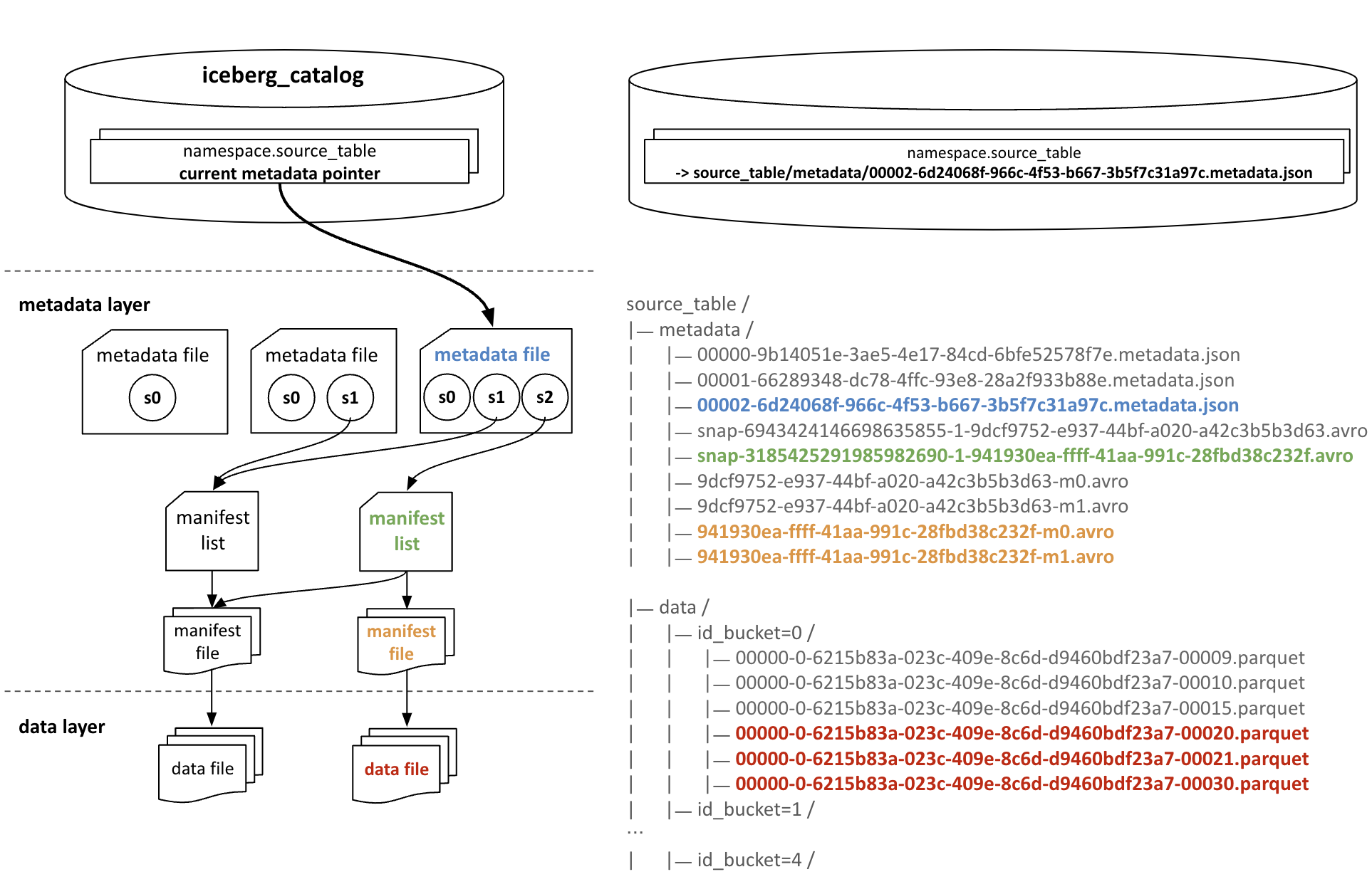
The generated files after the creation of the second snapshot are identical to those generated after the creation of the first snapshot. The difference is that the current metadata pointer now points to the newly created metadata file, which includes the new snapshot. Additionally, as shown in Example 11 , snapshot information with a sequence number of 2 has been added, and both the metadata and snapshot logs now each contain two entries. When a commit is performed and a new snapshot is created, the information from existing snapshots is accumulated in the latest metadata file. Based on these characteristics, Iceberg supports the time travel feature, which enables querying past states of the table. However, depending on the purpose and environment of using an Iceberg table, there may be no need to retain past snapshot information. Therefore, Iceberg provides a maintenance feature called Expire Snapshots. More detailed information about the Expire Snapshots feature will be explained in the subsequent section “Expire Snapshots and Delete Orphan Files”.
{
  "format-version" : 2,
  "table-uuid" : "884766bb-9cab-4298-829e-a096689d9ddc",
  "location" : "hdfs://hadoop-cluster/.../namespace/source_table",
  "last-sequence-number" : 2,
  ... // skip
  "snapshots" : [ {
    "sequence-number" : 1,
    "snapshot-id" : 6943424146698635855,
    "timestamp-ms" : 1723879779668,
    "summary" : {
      "operation" : "overwrite",
      "flink.operator-id" : "e883208d19e3c34f8aaf2a3168a63337",
      "flink.job-id" : "a40a5d923f750731620feafd9bf8930d",
      "flink.max-committed-checkpoint-id" : "1",
	  ... // skip
    },
    "manifest-list" : "hdfs://hadoop-cluster/.../namespace/source_table/metadata/snap-6943424146698635855-1-9dcf9752-e937-44bf-a020-a42c3b5b3d63.avro",
    "schema-id" : 0
  }, {
    "sequence-number" : 2, // new snapshot
    "snapshot-id" : 3185425291985982690,
    "parent-snapshot-id" : 6943424146698635855,
    "timestamp-ms" : 1723880377728,
    "summary" : {
      "operation" : "overwrite",
      "flink.operator-id" : "e883208d19e3c34f8aaf2a3168a63337",
      "flink.job-id" : "a40a5d923f750731620feafd9bf8930d",
      "flink.max-committed-checkpoint-id" : "2",
      ...
    },
    "manifest-list" : "hdfs://hadoop-cluster/.../namespace/source_table/metadata/snap-3185425291985982690-1-941930ea-ffff-41aa-991c-28fbd38c232f.avro",
    "schema-id" : 0
  } ],
  "statistics" : [ ],
  "partition-statistics" : [ ],
  "snapshot-log" : [ {
    "timestamp-ms" : 1723879779668,
    "snapshot-id" : 6943424146698635855
  }, {
    "timestamp-ms" : 1723880377728,
    "snapshot-id" : 3185425291985982690
  } ],
  "metadata-log" : [ {
    "timestamp-ms" : 1723879432267,
    "metadata-file" : "hdfs://hadoop-cluster/.../namespace/source_table/metadata/00000-9b14051e-3ae5-4e17-84cd-6bfe52578f7e.metadata.json"
  }, {
    "timestamp-ms" : 1723879779668,
    "metadata-file" : "hdfs://hadoop-cluster/.../namespace/source_table/metadata/00001-66289348-dc78-4ffc-93e8-28a2f933b88e.metadata.json"
  } ]
}
< Example 11: Metadata file created from the second snapshot >
Scan Planning and Maintenance of Iceberg
As previously explained, when loading data into Iceberg using Flink, data files and two types of delete files are generated. These files are merged to present a unified view when querying the Iceberg table. During this merging process, Iceberg references manifest lists and manifest files. In this section, I will explain which delete files are applied when querying an Iceberg table, what information is referenced, and how they are incorporated. I will also introduce Iceberg’s maintenance features that should be periodically executed.
Scan Planning
Scan planning is an optimization process that selects and combines the necessary data files and delete files using information from manifest files during a query. The information utilized includes the following, which will be explained in order:
-
Partition Information
-
Sequence Number
-
Statistical Information
The first information checked when incorporating delete files into data files is partition information . In the previous section, I explained that partition information is contained in the manifest files corresponding to data files and delete files. By using this information, data and delete files from the same partition are aggregated. This process allows for improved query performance by reducing the number of delete files applied to data files through proper partitioning. If a delete file lacks partition information, it is internally defined as globalDeletes and compared to all data files, negatively impacting performance.
The next information checked is the sequence number. It is incrementally assigned by one during snapshot creation and represents the relative age of snapshots shared by all files generated in the same snapshot. The conditions for comparing sequence numbers differ depending on the type of delete file, and these can be summarized as follows. Only delete files that satisfy these conditions are filtered:
-
Equality delete files: applied only to data files with a smaller sequence number, affecting only past snapshots.
-
Position delete files: applied to data files with the same or smaller sequence number, affecting up to the same snapshot.
For instance, in Example 1 , all values in the id column of the equality delete file exist in the id column of the data files because equality delete files are applied only to data files from earlier snapshots, as previously described. In other words, equality delete files affect only past snapshots, removing records with matching equality field column values from previous records and showing the latest records from recent data files during a query. A position delete file stores delete messages for records entered during the same snapshot. This applies to the case where the record with id=24 in Example 1 . After the record with id=24 arrived, a delete message for the same id arrived at the same snapshot time. Thus, the record with id=24 should not appear in the result of the query, the position delete file is designed to apply up to the same snapshot.
Finally, equality delete files take the process one step further by utilizing statistical information about the equality field columns. This statistical information includes the minimum and maximum value information for the equality field columns, which is used to compute the range of equality field column values within each file. Only delete files with overlapping equality field column ranges with the data files are ultimately applied. Figure 14 illustrates the entire process for a data file with a sequence number of 1 and a partition of 0, showing how equality delete files that are to apply are selected. Through these processes, Iceberg ensures that only the minimum necessary delete files are applied to data files, and presents the results to the user.
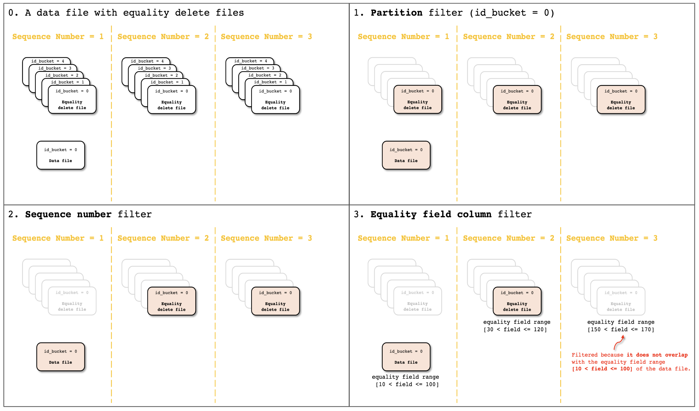
Compaction
Compaction is a maintenance feature that combines data files and delete files into large new data files. As previously explained, when loading data into an Iceberg table using Flink, the data is stored in data files and two types of delete files. Additionally, new files are generated with each checkpoint, as CDC (Change Data Capture) continues to collect change data; thus, the number of files increases over time. Consequently, query time will inevitably continue to increase over time as more files are generated.
Of course, as noted in the section “Flink Configuration”, we can extend the checkpoint interval to reduce the frequency of file creation. However, this only decreases the rate at which query time increases, and it doesn’t address the fundamental cause of increased query times due to the growing number of files. Therefore, the fundamental way to reduce table query time is to use the compaction.
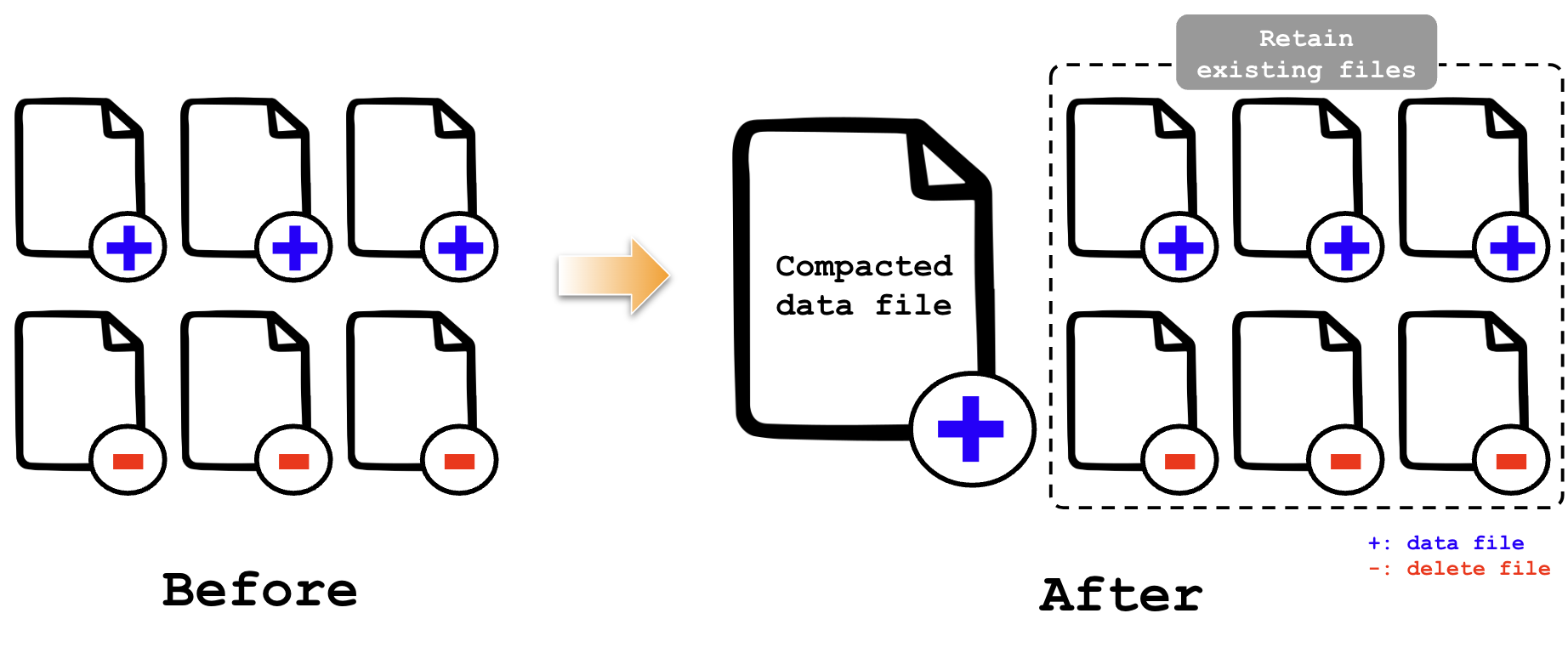
The following Graph 1 illustrates the trend of how table query time increases without performing compaction. The table used in the test contains 3 billion records, with an average of 4 million changes per day. Flink’s checkpoint interval is set to 10 minutes, resulting in file creation every 10 minutes. Spark was used for table queries, with 1,000 executors and 48GB memory allocated per executor. As seen in Graph 1, immediately after CDC integration (day 0), querying the entire table took merely 2.8 minutes, but after a week, the query time increased to 60 minutes. Finally, after performing compaction on the seventh test day, the compaction took 39 minutes, and querying the entire data took 1.7 minutes. This result suggests that the compaction is an essential feature for keeping query times short when operating an Iceberg table.
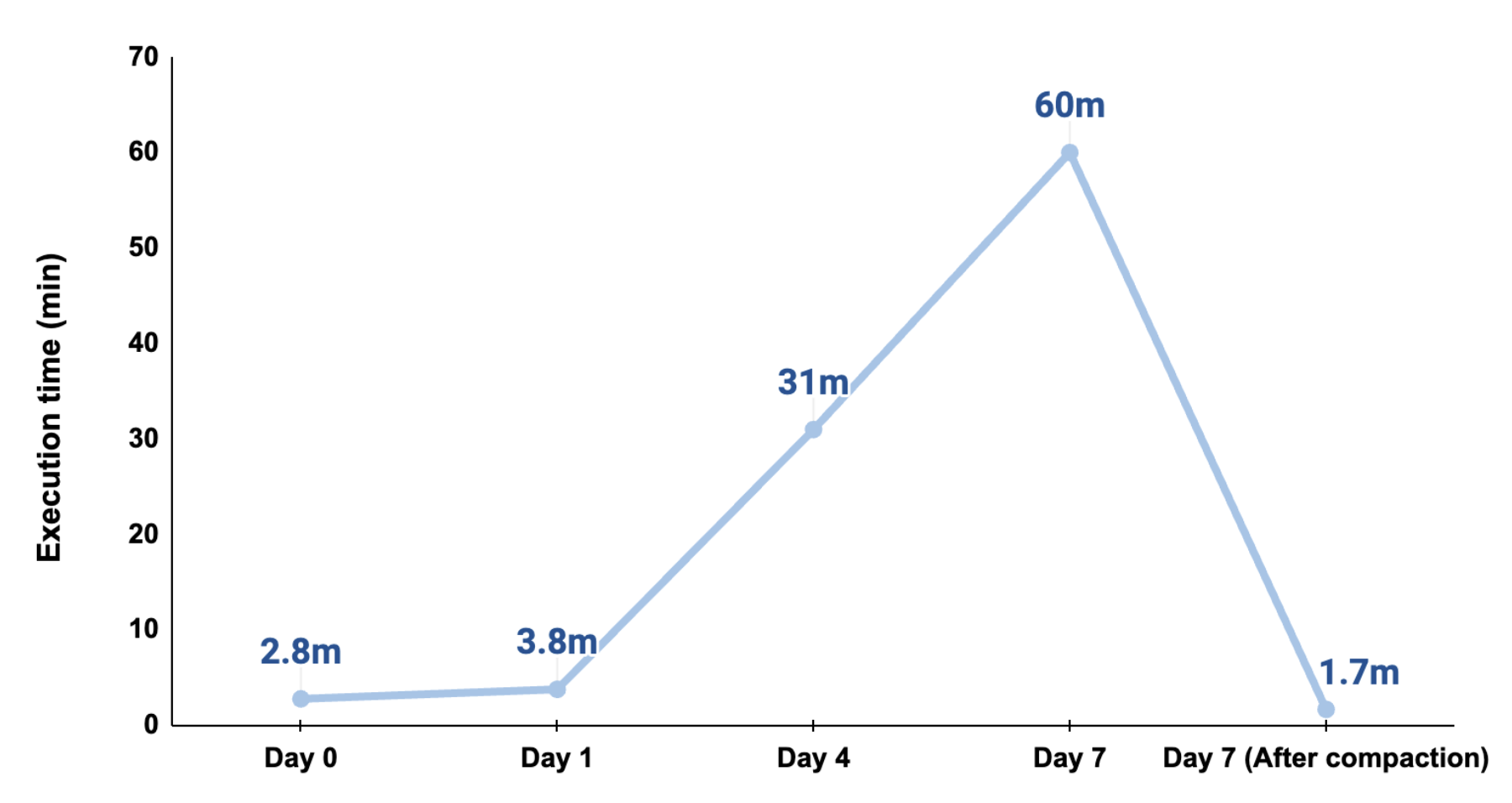
Next, I share a specific scenario to watch out for during compaction. Data files that have already been compacted may be excluded from subsequent compactions under certain conditions. The options related to this are min-file-size-bytes and max-file-size-bytes. If, due to these settings, the size of a compacted data file falls within 0.75 to 1.8 times the target-file-size-bytes configured by the user, those files will be excluded from further compaction operations.
For example, in a situation our team encountered, when target-file-size-bytes was set to 250MB, data files compacted to between 187.5MB and 450MB were excluded from future compaction tasks. As a result, delete files created after these data files, which were compacted to sizes between 187.5MB and 450MB, remained referenced because of the presence of the preceding data files. Therefore, even when performing expire snapshots and delete orphan files, discussed later, these files were not deleted as they remained referenced, leading to a situation where over 40,000 small delete files continued to accumulate as shown in Figure 16 . To resolve this issue, our team set the rewrite-all option in compaction to true, ensuring that all data files are always considered as candidates for compaction.
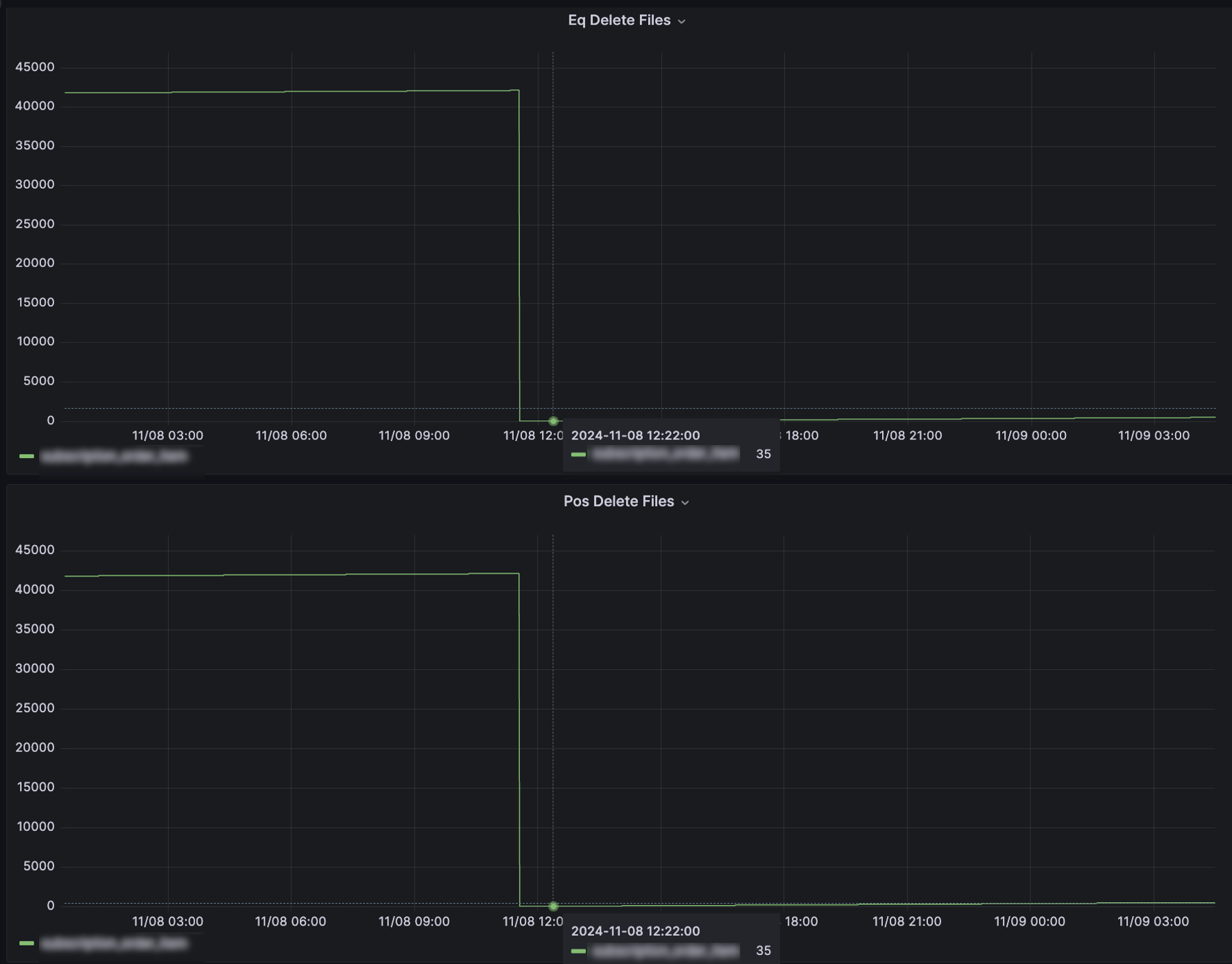
Finally, I would like to share a metric we use to evaluate whether compaction will take a long time. Compaction is a process that combines files to improve table query speeds, performing tasks similar to sourcing tables. Therefore, compaction takes considerable time.
While we can’t identify all factors and correlations affecting compaction time at this point, we focus on the types of changes entering the table based on our experience with various tables. Empirically, tables with a high ratio of update queries in change events tend to take more time for compaction, even with the same number of change events. However, we haven’t tested this case due to difficulties in finding tables where the number of records and changes are similar but the query type ratio varies significantly.
Instead, we tested tables with different record counts but similar change counts and varying query type ratios. The test tables contain 3 billion and 90 million records, respectively, with both tables averaging 4 million changes per day. We measured the time taken for compaction using Spark, setting up 500 executors and allocating 16GB of memory per executor. Table 1 below summarizes the results for both tables.
| 3B Records Table | 90M Records Table | |
|---|---|---|
| INSERT Query Count & Ratio | 1.7M (42%) | 0.09M (2.2%) |
| UPDATE Query Count & Ratio | 2.1M (53%) | 3.88M (96.3%) |
| DELETE Query Count & Ratio | 0.2M (5%) | 0.06M (1.5%) |
| Avg Compaction Time for daily changes | 5 min | 9.7 min |
< Table 1: Comparison of query types ratio and compaction time >
As seen in Table 1, the table with 90 million records took longer for compaction, even though the difference in the number of records was 30 times. We focused our analysis on the fact that about 53% of the changes were update queries for the 3 billion record table, while about 96% for the 90 million record table. Our analysis may not be perfect or definitive, but based on our understanding of Iceberg’s architecture and operation, here is what we found:
Both insert queries and update queries store data in data files and delete files. The difference is that insert queries contain newly assigned equality field column values, while update queries update existing records and consequently have already existing equality field column values. Therefore, higher proportions of update queries result in more data stored in position delete files. However, as explained in the section “Scan Planning ”, position delete files do not benefit from maintenance using equality field column ranges. Consequently, since more data stored in the position delete file, and position delete files compared to more data files than equality delete files, we interpret that higher proportions of update queries negatively impact execution time.
Expire Snapshots and Delete Orphan Files
The next maintenance features to consider are Expire Snapshots and Delete Orphan Files. As previously explained, Iceberg’s metadata files retain information on all snapshots. Expire Snapshots maintains only snapshots up to a user-specified point in time and deletes older ones. Essentially, it removes the information on snapshots that are older than a certain point from the metadata files.
However, Expire Snapshots only removes references and does not delete the actual files. The feature responsible for deleting files without references is the Delete Orphan Files. This feature doesn’t delete all unreferenced files; like Expire Snapshots, it deletes unreferenced files older than a user-specified point in time. If you set the same point in time for both features, they will retain snapshots up to that point and delete older snapshots and files.
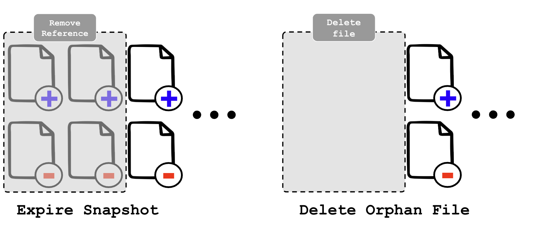
That said, because these features affect the range of dates accessible through the time travel feature, you must set an appropriate point in time if you plan to use it. Performing Expire Snapshots means that you cannot query table states from before the expiration point. Therefore, if you expect to query tables for states up to 6 months in the past using time travel, you should set the time condition for Expire Snapshots and Delete Orphan Files to at least 6 months.
Our team, not using the time travel feature, established different retention criteria for files. For sensitive data with security concerns, even if hashed or masked, there were frequent requests to delete data periodically. Thus, to make past states inaccessible and delete outdated data, we performed Expire Snapshots and Delete Orphan Files at short intervals. While general data did not present security issues, we were using HDFS for object storage, and frequent creation of small files negatively affected Hadoop’s IO performance due to Hadoop block size. Consequently, we also configured Expire Snapshots and Delete Orphan Files for general data at short intervals to align with our team’s needs.
Moreover, these maintenance features need to be executed periodically. To handle this, our team uses Apache Spark for maintenance jobs and orchestrates them through Apache Airflow.
In addition to the maintenance described in this article, other maintenance features such as Rewrite Position Delete Files and Rewrite Manifests exist to optimize position delete files and manifests. It is recommended to select the appropriate maintenance according to your own environment and purpose.
Integrating Sharded Table into a Single Iceberg Table
In this section, I will share the process of testing whether sharded tables can be integrated into a single Iceberg table and operated. The test examined whether sharded tables can be physically integrated into one Iceberg table, whether there are performance improvements and operational benefits when extracting metrics, and whether stable operation is possible. First, the benefits of integrating into a single table are as follows:
-
Simplification of metric extraction by integrating multiple table sourcing tasks into a single table sourcing task
-
Elimination of the union process to merge sourced tables
-
Simplification of maintenance tasks (compaction, expire snapshots, delete orphan files) into operations on a single table
Design and Implementation
The approach to implement this is to maintain a structure where the way data is stored and queried from each Iceberg table remains physically and logically similar. This is to minimize the additional load that may occur when integrating into a single Iceberg table.
To achieve this, sharded tables are stored as separate partitions. The reason for partitioning is that the merging of data files and delete files when querying the table is performed for each partition, as explained in the section “Scan Planning ”. Therefore, if sharded tables are loaded only into each partition, the data and changes of each sharded table are physically separated and stored in partitions. As a result, each partition only processes the data and changes of one sharded table. Figure 18 shows an example of this partition structure.
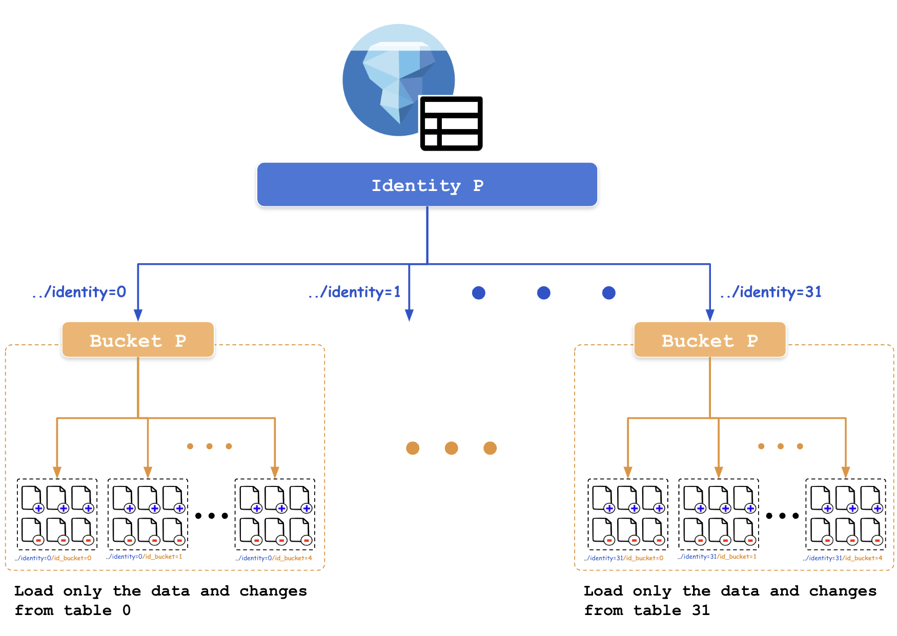
Now, I will explain how partitions are set. First, sharded tables are separated into partitions through identity partitioning. Then, within each partition, a bucket partition is performed to match the structure when integrating a single table to an Iceberg table. For this reason, identity partitioning and then bucket partitioning are sequentially set, and the detailed steps are as follows:
-
Add a
shard_numbercolumn to store the shard number when creating the Iceberg table -
Add the
shard_numbercolumn to the equality field columns -
Sequentially set identity partitioning on the
shard_numbercolumn and bucket partitioning on the primary key (e.g.,id)(e.g., …/identity={shard_number}/id_bucket=0/…, …/identity={shard_number}/id_bucket=1/…)
-
Add the shard number dynamically to the messages transmitted when loading data into the Iceberg table from Flink
As explained based on Figure 18 , the numbers in the form identity=? represent the shard number assigned to each sharded table. Within the identity partition, data is stored in a structure like ../identity=0/id_bucket=4 through bucket partitioning. In summary, the data of each sharded table is distinguished by identity partitions, preventing additional operations such as merging data that may occur during table queries when the data of sharded tables mixes. In addition, by adding the bucket partition under the identity partition, we maintain efficient table query performance. For the configuration of each sharded table loaded into an Iceberg table through Flink jobs, please refer to Figures 19 and 20.
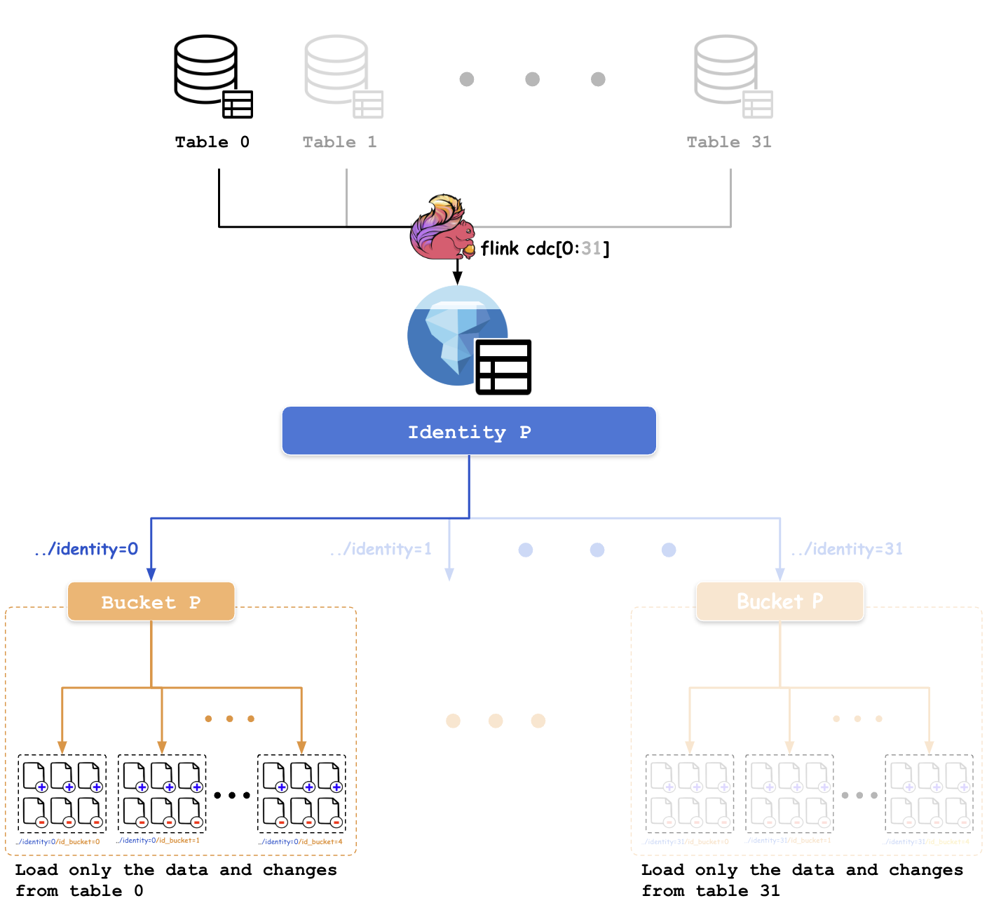
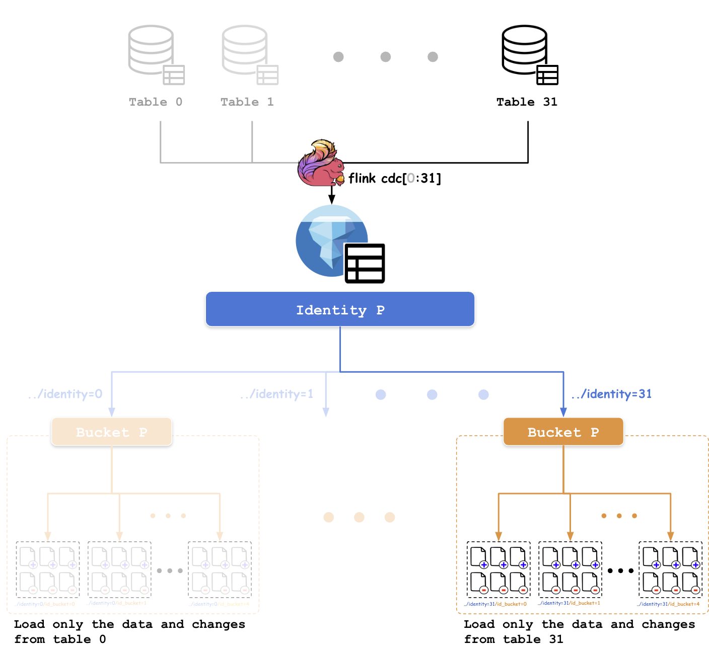
Test
We loaded 32 tables containing a total of 2.7 billion records into a single Iceberg table. Then, compaction and entire table data sourcing were performed through Spark, and we measured the time taken for sourcing. The test results showed that it took an average of 270 seconds, and for comparison, sourcing an Iceberg table with 90 million records took an average of 20 seconds. By comparing the execution of 32 tasks each taking 20 seconds, we could see that our approach was more efficient in terms of performance.
Limitation
However, it was judged to be unstable and thus could not be applied to the production service. Because, multiple flink jobs perform commits periodically to a single Iceberg table.
The reason for this instability is as follows. Commits are performed based on the base metadata file, and once a commit is completed, the base metadata file is updated. The base metadata file refers to the file that the current metadata pointer indicates. If multiple commits are performed on a single table simultaneously, only one flink job completes the commit. The remaining flink jobs will encounter Error Message 2 when attempting their commits, because the base metadata file they are referencing has changed before they complete their commits.
org.apache.iceberg.exceptions.CommitFailedException: Cannot commit: Base metadata location 'hdfs://../../namespace/table/metadata/XXX-A.metadata.json' is not same as the current table metadata location 'hdfs://../../namespace/table/metadata/XXX-B.metadata.json' for namespace.source_table
< Error Message 2: Commit conflicts >
Continuing explanation with Figure 21 as an example
First, both the 0th flink job and the 31st flink job perform commits based on the base metadata file XXX-A.metadata.json. Once the 0th Flink job completes its commit, the updated current metadata pointer indicates the newly created metadata file, XXX-B.metadata.json. As a result, the 31st Flink job encounters an error because the base metadata file has changed before it could complete its commit.
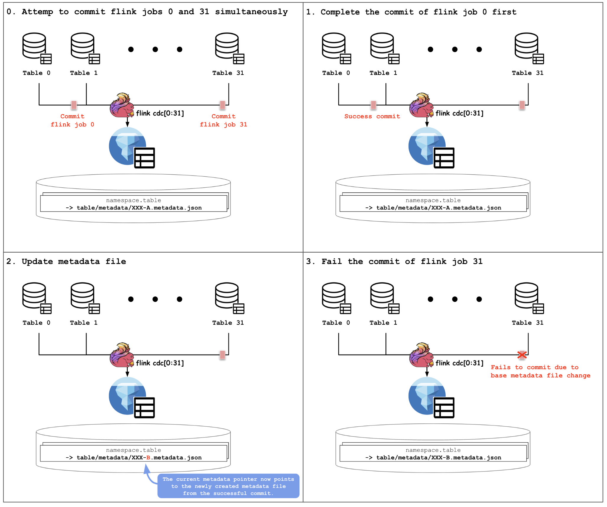
Of course, even if such an error occurs, a flink job does not stop immediately. An option COMMIT_NUM_RETRIES related to this error already exists within Iceberg, allowing a flink job to not stop if it successfully commits within a maximum retry count even after a failure. A test conducted internally demonstrated this by adjusting the retry count to 60, observed over a week. Although some flink jobs out of 32 encountered commit failures, none of them stopped due to exceeding the maximum retry count.
However, among the tables requiring CDC integration to Iceberg, there are tables that are sharded with more than 100 tables. And simply increasing the maximum retry count was not enough to ensure stability. In particular, since stability is as important as performance in the production service, we could not apply this feature that could potentially stop a flink job. As an alternative, we discussed applying this to tables with fewer shards. But we decided to maintain the same policy for all sharded tables, and ultimately decided not to apply this feature.
Conclusion
I would like to express my sincere gratitude to the readers who have been with me until the end of this long article, and I would like to conclude with some personal thoughts.
Firstly, I think that the process of loading data into Iceberg through Apache Flink was not an easy task. It was the first time that the team introduced data lakehouse technology, and it seems that applying CDC to Iceberg through Flink is still rare in Korea. There are a few oversea cases, they were slightly different from our team’s requirements at the time. For example, there were many cases where Flink SQL was used instead of Flink’s DataStream API, or S3 was used as object storage instead of the Hadoop file system.
Also, since I had no understanding about the operation process of Iceberg at first, I had to figure out how data was loaded and what information was in the files. To do this, I had to deeply analyze the system and library code, perform tests, and examine the generated files one by one. Although these processes were not easy, I found them to be a meaningful and rewarding experience because it allowed me to share more in-depth content with readers, thanks to how I carefully organized and documented this journey.
Finally, I hope this article serves as a milestone for those who are considering conducting CDC using Flink and Iceberg, and also satisfies the curiosity of those who simply explored this article.
Thank you.