Engineering
Iceberg Operation Journey: Takeaways for DB & Server Logs
louis.sml카카오
2025년 4월 18일
원문에서 보기 ↗Hi, I am SeungMin Lee from the Data Analytics Platform team at Kakao.
This is the last article in the series. In the first article, we shared performing CDC (Change Data Capture) using Apache Flink to synchronize a MySQL table with another MySQL table, and in the second article, we shared our experiences gained from performing CDC from MySQL tables to Apache Iceberg and operating the system. In this article, we intend to share how best to perform partitioning and optimization for Iceberg tables based on the type of logs being collected, along with our current operational methods and the results of our tests.
First, to briefly state our team’s mission, it is to retrieve data from service teams to extract and provide daily metrics. We collect data from diverse sources, including Apache Kafka and databases, and in this process, there are cases where we need to access data from the service teams’ databases. However, as the approach of accessing service teams’ databases to retrieve data could affect the production services, we have improved the metrics extraction pipeline by integrating with Iceberg, one of the data lakehouse technologies, via CDC, as demonstrated in the first article.
This article aims to share the necessary settings and optimal operational methods when loading two types of logs into Iceberg tables. First, we introduce the method of loading logs collected for metrics extraction into Iceberg tables according to their type and characteristics. Then, we share our experiences with partitioning strategies and optimization methods for Iceberg tables, considering the loaded data and query patterns. Finally, we conclude the article by summarizing how to monitor Iceberg-related metrics.
If you are unfamiliar with Apache Flink and Iceberg, you might find this article a bit challenging to follow. Therefore, we recommend first reading the second article, which covers the basic concepts of Iceberg.
Log Types and Collection Methods
Our team utilizes the following types of logs for metrics calculation:
- Client Logs
- Server Logs
- Database Change Logs (DB Logs)
Among these, server logs and DB logs are directly collected by the team and utilized for calculating metrics. In this section, regarding DB logs, we will introduce the current operational methods. Regarding server logs, we will share our current collection method and the details of the tests conducted to improve it.
However, we would like to state in advance that the method for DB logs is currently applied in the production environment, while the approach for server logs represents a direction currently under testing . Please note that depending on the specific purpose and environment, there may be more optimal settings or methods than those discussed in this article.
DB Logs
As mentioned in a second article, for DB logs, we are synchronizing MySQL tables from various service teams to Iceberg tables within our team’s Hadoop File System (HDFS) using Apache Flink for Change Data Capture (CDC). We will briefly share the details regarding write mode, partitioning strategy, and commit interval for the Iceberg tables currently in operation.
We are loading data into the Iceberg tables using the UPSERT mode, based on the Primary Key (PK) of the corresponding MySQL tables. This approach ensures that the latest data, reflecting continuous changes in the MySQL tables, can be queried directly from the Iceberg tables. Furthermore, to optimize performance for queries and compaction, we apply bucket transform partitioning based on the Primary Key. This enables effective data pruning to avoid reading unnecessary data.
The commit interval is aligned with the Flink job’s checkpoint interval and is set to 10 minutes. This setting aims to minimize the small file issue while maintaining proper data freshness. As a result, we no longer need to source the entire MySQL table data daily. Additionally, there is no need to limit the performance of Spark applications due to concerns about the MySQL server load. Consequently, we can now allocate resources to Spark applications as needed, significantly reducing the data sourcing time.
Server Logs
Server logs refer to the logs generated by the servers within each service team. Since these logs originate from various servers specific to each service, their format and structure often vary across different service teams. We request service teams to send their logs via Apache Kafka, conforming to the JSON specification defined by our team, like the example in Figure 1 below. Then we use Apache Flink to consume these logs from Kafka and store them in our team’s Hadoop cluster in the ORC format.
{
	"cluster_name": "...",
	"host": "...",
	"meta": {..},
	"log": "{..}",
	"log_format": "json"
}
Figure 1. Json Specification
During log loading, the Flink job adds a process time value. We store the logs using daily and hourly partitions based on this time. We do not use event time and watermarks to ensure idempotency, meaning final metrics remain unchanged even during data reprocessing. However, this method might place some late data into partitions later than their actual event date. We correct these exceptions later during the Spark sourcing stage.
The ORC format and the current collection method have been used by the team for a long time. They operate without major issues currently. However, DB logs are already synchronized to Iceberg via CDC. Therefore, we considered loading server logs into Iceberg using APPEND mode. This would unify the data format sourced by Spark to Iceberg and also allow building a consistent monitoring system for both DB and server logs.
The reason that we chose APPEND mode is that UPSERT could leverage the unique IDs in server logs to remove duplicates, but the amount of server logs is too large, so the optimization cost is too high compared to the benefit. Furthermore, since duplicate removal is handled later during the Spark metric calculation stage, anyway. Therefore, considering the amount of server logs, the number of data and deleted files, and the related optimization cost, APPEND mode was chosen.
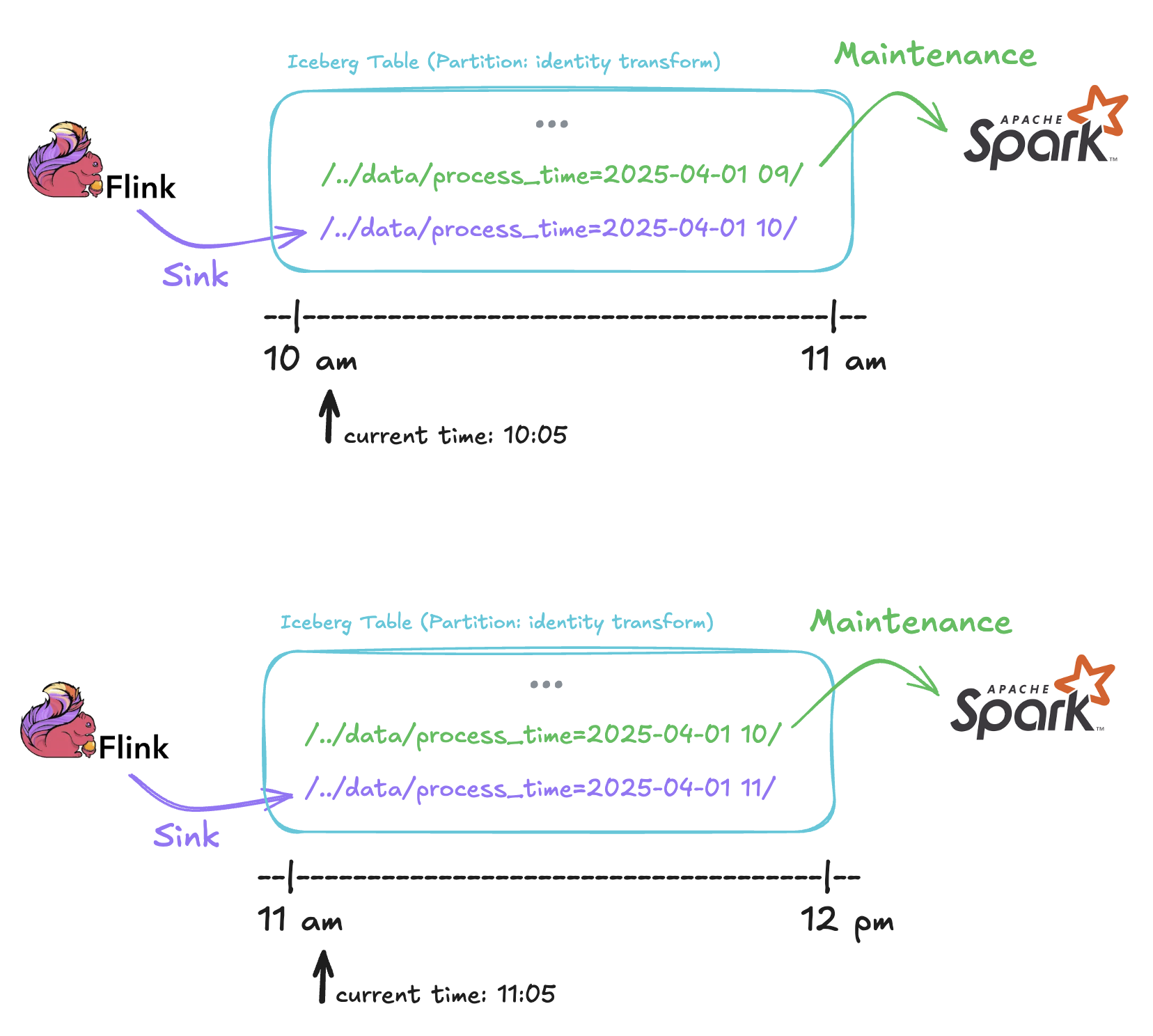
We are also considering shortening the Flink job’s checkpoint interval (currently 3 minutes). This aims to reduce the Kafka Lag Count. However, frequent checkpoints create smaller files. This leads to the small file problem, negatively impacting HDFS and Spark sourcing performance. To address this, we apply identity transform partitioning on the hourly time (process time) value . Additionally, as depicted in Figure 2 below, we run Iceberg’s optimization features hourly on the previous hour partition.
This means using compaction to merge small files into larger ones. We also use snapshot expiration and delete orphan files to delete unneeded small files. This allows shortening the checkpoint interval (reducing Kafka lag). At the same time, Iceberg’s optimization manages file size and count optimally, so we can improve both storage usage and query performance. We will share more details in a later section.
Compression, Partition and Optimization Strategies
There are three major factors to consider when utilizing Iceberg:
- Format & Compression
- Partition
- Compaction, Expire Snapshots, Delete Orphan Files
In this section, we will share how we are currently utilizing and operating the three aforementioned methods for DB logs, and the results of our tests regarding how we plan to improve for server logs cases.
Compression
Iceberg’s default file format is Parquet. Since version 1.4.0, its default compression codec has been zstd, reportedly changed from gzip to achieve better compression performance and address potential gclocker-related issues. Also, since we source our data using Spark, we continue using Parquet as the file format due to its excellent compatibility with Spark, regardless of the log type. For compression, when we initially set up CDC for DB logs into Iceberg, their volume was significantly smaller compared to server logs. Consequently, we simply used the default settings – zstd compression with level 3 – without extensive analysis at that time.
However, server logs generate at least tens of times more volume than DB logs, necessitating a careful consideration of compression settings. While we decided to use the default zstd codec, we needed to test different compression levels**. We tested different compression levels with a Kafka topic that receives an average of 3 billion server logs per day and 50,000 per second**. The key aspects we evaluated in these tests were:
- Whether the CPU usage ratio changed with varying compression levels.
- Whether any processing latency occurred.
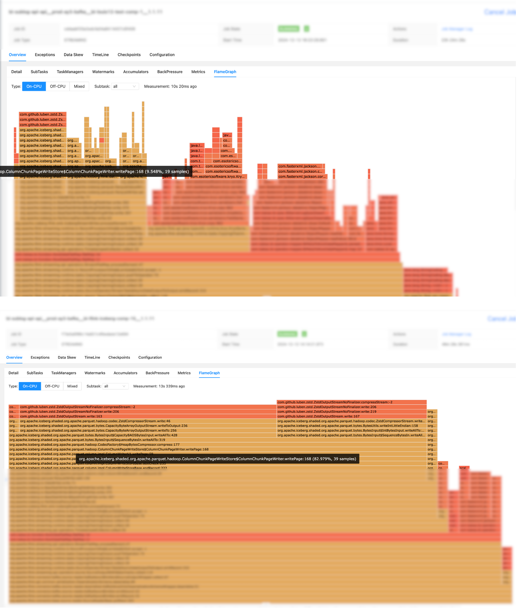
If higher compression levels lead to increased CPU usage ratios and potentially cause latency, their adoption requires careful consideration. To investigate this, we measured the CPU usage ratio specifically associated with zstd compression at different levels. We achieved this by enabling FlameGraph within Flink and observing the CPU usage ratio of compression-related methods. The results, as shown in Table 1 below, indicated a clear trend: the CPU usage ratio attributable to compression significantly increased as the compression level rose . Despite this, we observed no significant difference in the overall CPU utilization of Flink Task Manager pods.
| Compression Level | Level 1 | Level 3 | Level 6 | Level 9 | Level 12 | Level 15 |
|---|---|---|---|---|---|---|
| CPU Usage Ratio | up to 10% | 9 ~ 14% | 18 ~ 27% | 29 ~ 38% | 41 ~ 53% | 75 ~ 84% |
Table 1. CPU Usage Ratio by zstd Compression Level
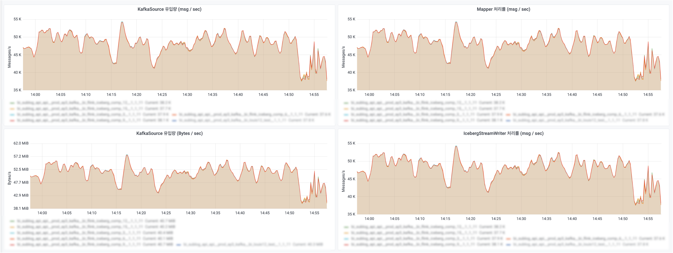
Although we confirmed that there was no significant difference in the CPU utilization of individual Task Manager Pods despite the increased CPU usage ratio, it is also necessary to verify whether latency occurs during the actual data loading process. If latency is determined to exist in Iceberg table loading, we must reconsider whether it is applicable in the production environment. Accordingly, based on the same Kafka topic used in the previous tests, we analyzed the following metrics from Kafka and Flink perspectives to determine whether latency exists:
- Kafka Perspective: Difference in the number of messages consumed and committed to Kafka over 4 hours.
- Kafka Perspective: Difference in the decrease in Kafka’s Lag Count over 1 hour.
- Flink Perspective: Throughput (msg / sec).
First, from the Kafka perspective, we examined the difference in the number of messages consumed and committed over 4 hours and the decrease in Lag Count over 1 hour. The test results are shown in Table 2 below. Summarizing the cases with the largest differences observed between compression levels:
- Number of committed messages: Approximately 0.6% difference between compression levels 9 and 6.
- Decrease in Lag Count: Approximately 0.3% difference between compression levels 6 and 15.
Kafka commits are performed according to the Flink job’s checkpoint interval, and even if the interval is the same, differences can occur in the exact commit timing. Considering this, in our case, although the CPU usage ratio increases by up to 84% as the compression level increases (as shown in Table 1), we concluded that latency was negligible.
| Compression Level | Level 3 | Level 6 | Level 9 | Level 12 | Level 15 |
|---|---|---|---|---|---|
| Number of Committed Messages (4h) | 555.68M | 553.44M | 556.60M | 554.48M | 555.50M |
| Lag Count Decrease (1h) | 128.50M | 128.32M | 128.67M | 128.42M | 128.73M |
Table 2. Number of Committed Messages and Lag Count Decrease by Compression Level
Then, to check for latency from the Flink perspective, we measured the throughput of the Flink job. For reference, the Flink job used in the test was configured according to internal team policy, which requires minimizing the transformation of source data to facilitate reprocessing. Therefore, it was set up to operate by consuming logs from Kafka without complex operations, parsing them using the Jackson library, and then converting them into the RowData format used for Iceberg table loading.
The test results are shown in Table 3 below. Within the same compression level, the throughput was nearly identical. Furthermore, the change in throughput due to changes in the compression level was also minimal, with the maximum difference being only about 0.3%. Considering these results comprehensively, although the CPU usage ratio increased with the compression level, there was no significant difference in the CPU utilization of individual Task Managers, and no latency occurred from either the Kafka or Flink perspectives . Therefore, we concluded that the effect of compression level on overall performance is not significant, and the likelihood of actual latency occurring due to the increased compression level is low.
| Compression Level | Level 3 | Level 6 | Level 9 | Level 12 | Level 15 |
|---|---|---|---|---|---|
| Throughput(msg / sec) | 46,456 | 46,437 | 46,426 | 46,339 | 46,602 |
Table 3. Flink Job Throughput by Compression Level
Now that we’ve confirmed that latency was negligible, we examined the benefits of loading compressed server logs into Iceberg tables. One of these is the impact of increased compression levels on file size reduction, which we tested and compared. However, one thing to consider when interpreting the results is the difference in checkpoint intervals: the current Flink job loading data in ORC format has a 3-minute checkpoint interval, while the test Flink job for loading Iceberg tables has a 1-minute checkpoint interval . As mentioned earlier, the reason for reducing the checkpoint interval to 1 minute was to reduce the Kafka Lag Count through more frequent checkpoints.
Also, considering how Iceberg tables work, leaving many small files is not good for the performance of queries or optimization features. Therefore, the process of combining small files into larger ones and deleting the small files is important. This optimization method will be explained in detail in the subsequent sections “Partition” and “Optimization Strategy”.
Table 4 below shows the calculated daily file size (for a weekday) by compression level when consuming the Kafka topic that receives an average of 3 billion server logs per day. It also summarizes how much the file size was reduced compared to the daily file size (750.3 GB) of server logs loaded using the existing ORC file format, specifically compared to compression levels 1 and 3 (the default).
| Compression Level | Level 1 | Level 3 | Level 6 | Level 9 | Level 12 | Level 15 |
|---|---|---|---|---|---|---|
| Daily File Size (GB) | 473.4 | 453.5 | 402.9 | 364.4 | 358.1 | 347.1 |
| Reduction Ratevs. ORC Format (750.3 GB) | 36.9% | 39.6% | 46.3% | 51.4% | 52.3% | 53.7% |
| Reduction Ratevs. Level 1 (473.4 GB) | N/A | 4.2% | 14.9% | 23.0% | 24.4% | 26.7% |
| Reduction Ratevs. Level 3 (453.5 GB) | N/A | N/A | 11.2% | 19.6% | 21.0% | 23.5% |
Table 4. Daily File Size and Reduction Rate by Compression Level
It’s important to note, however, that these compression ratios are not consistent in all situations. The compression ratio can vary depending on the volume of server logs generated, and the results presented above correspond to cases with a relatively high volume of logs. To further investigate this, we conducted tests using compression level 9 on Kafka topics that handle a significantly lower volume of server logs. The results are shown in Table 5 below. As expected, the topic averaging 3 billion logs per day exhibited the highest size reduction rate at approximately 51.4%, whereas topics with lower volumes showed average reduction rates ranging from 23.9% to 31.8%.
| Daily Server Log Volume | Reduction Ratevs. ORC Format(at Level 9) |
|---|---|
| 3 Billion | 51.4% |
| 90 Million | 27.7% |
| 20 Million | 23.9% |
| 2 Million | 31.8% |
Table 5. Reduction Rate by Daily Log Volume
When interpreting these test results, it is important to clearly distinguish whether this reduction effect is due to the Iceberg table itself, or simply due to the use of Parquet file format and the zstd compression codec. In other words, it is necessary to verify if there is a difference compared to the previous results when server logs are loaded directly using the Parquet file format and zstd compression codec, without using an Iceberg table.
The test results showed no significant difference in file size between loading data into an Iceberg table using the Parquet format and zstd codec, and loading it directly using the same format and codec. Table 6 below presents the results of a test conducted on server logs averaging 3 billion per day. The file size using the Parquet format with zstd compression (469.1 GB) was nearly identical to the size when loading into an Iceberg table using the same format and codec at compression level 3 (469.6 GB). Please note that there might be slight differences compared to the previous Table 4 due to differences in the test execution dates.
Therefore, the aforementioned file size reduction can be interpreted as a benefit derived primarily from using the Parquet file format and the zstd compression codec, rather than specifically from loading the data into an Iceberg table.
| ORC | Parquet & zstd | Parquet & gzip | Iceberg (Level 3) | Iceberg (Level 6) | Iceberg (Level 9) | |
|---|---|---|---|---|---|---|
| Daily File Size (GB) | 799.4 | 469.1 | 590.9 | 469.6 | 418.5 | 379.6 |
| Reduction Ratevs. ORC Format | N/A | 41.3% | 26.1% | 41.3% | 47.6% | 52.5% |
Table 6. File Size Comparison: Iceberg Table vs. Direct Parquet & zstd / gzip
Finally, we tested whether there was a difference in the time it took to source the Iceberg table in Spark for a day depending on compression level. This test was also performed using server logs averaging 3 billion per day. The Spark configuration was fixed with 32 executors, each allocated 4GB of memory. Additionally, please note that no separate optimization, such as compaction, was performed.
The results showed a slight increase in sourcing time as the compression level increased. There was a difference of approximately 4 minutes, representing about a 10% increase in time, between compression levels 3 and 9. However, it should be considered that compaction was not performed in this test, more resources can be allocated in a production environment, and data is usually sourced on an hourly basis rather than an entire day’s worth at once. Consequently, the difference is expected to be significantly smaller in a production environment, even with increased compression levels. Therefore, we concluded that this should not pose a significant issue for Spark sourcing operations.
| Level 1 | Level 3 | Level 6 | Level 9 | Level 12 | Level 15 | |
|---|---|---|---|---|---|---|
| Average Sourcing Time (min) | 37.8 | 37.2 | 38.4 | 41.6 | 40.8 | 40.6 |
Table 7. Average Spark Sourcing Time by Compression Level
Partition
Iceberg’s partitioning and optimization strategies are key factors that directly impact query performance. In this section, we share our approach to load data into Iceberg tables and the optimization strategies applied, considering the specific characteristics of DB logs and server logs. Before we delve into the details, Table 8 below summarizes the write mode, partition, and optimization frequency for each log type.
| DB Logs (Production) | Server Logs (Testing) | |
|---|---|---|
| Write Mode | UPSERT | APPEND |
| Partition Transform | Bucket transform on PK Column(bucket size = 5) | Identity transform on process time column |
| Optimization Interval | Two per day (morning, afternoon) | Hourly |
Table 8. Iceberg Table Configuration by Log Type
For DB logs, which experience frequent updates and deletes, we loaded them using UPSERT mode based on the Primary Key column and applied a bucket transform partition to enable efficient querying. Additionally, we maintain performance by running optimization twice a day.
In contrast, server logs primarily involve new data being added, so we tested using the APPEND mode. Our Flink job adds a process time column and value to these logs, similar to our existing Flink job that writes to ORC format. However, for Iceberg, this process time is stored as a string type, omitting units smaller than an hour (like minutes and seconds).
Using time-related column types (like Timestamp) and applying an hour transform partition would allow for hourly partitioning. However, this introduces challenges with timezone differences. Iceberg inherently treats stored timestamp-related values as UTC. The goal within the Iceberg community is to provide consistent values regardless of where the data is queried. Therefore, Iceberg always assumes and stores time-related column values in UTC; timezone conversions must be handled by processing engines like Spark or Trino.
Although our Flink job generates the process time based on KST (Korea Standard Time), when this value is stored in Iceberg, the literal value doesn’t change, but Iceberg interprets it as being in the UTC timezone. This creates a problem because our team’s Spark sessions are configured for KST. When these sessions read the value stored as UTC, they convert it to KST by adding +9 hours, resulting in an incorrect timestamp being returned.
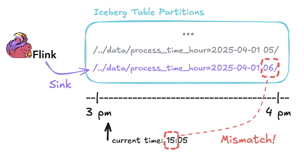
To resolve this, we could subtract 9 hours when generating the process time. However, even if there is no problem with reading the data with Spark, this creates another problem when applying an hour transform partition on the process time column. This is because the data would be loaded into a partition corresponding to 9 hours before the actual processing time . For instance, as illustrated in Figure 5 below, a log processed at 15:00 on April 1st, 2025 (KST) would incorrectly be placed in the partition for 06:00 on April 1st, 2025 (../data/process_time_hour=2025-04-01 6).
During testing, we chose to avoid timezone problems by storing the process time in a string type column, as mentioned earlier. Also, since time-related transforms like day and hour require time-related column types (like Timestamp), we applied the identity transform to the process time string column to make it behave the same as the hourly partition.
Optimization Strategy
Iceberg has important optimization features like Compaction, Expiring Snapshots , and Delete Orphan Files . In this section, we will explain the optimization strategy we use now for DB logs in production , and the method we tested for server logs.
First, for the strategy option for compaction, we use the default binpack strategy for both log types. We chose this because of how our team usually uses these Iceberg tables: Iceberg tables for DB logs mainly perform full table scans, while Iceberg tables for server logs mainly perform scans for the previous day. So, we didn’t choose strategies like sort or z-order, which are better for queries that filter using specific columns.
Also, we set the rewrite-all option to true for compaction. This makes sure all files can be rewritten during compaction. If we didn’t set this (rewrite-all=true), files whose size is between 0.75 and 1.8 times the target-file-size-bytes would be skipped by compaction because of the default min-file-size-bytes and max-file-size-bytes settings. If files are skipped, some delete files might keep being referenced, which might stop old data from being removed even after the set retention period.
Also, we set partial-progress.enabled to true. This lets Iceberg save progress (commit) even while compaction is running. However, since this feature is useful for improving query performance by utilizing intermediate results of the compaction for queries performed during the compaction process, it is recommended to set it to false if there is no need to run queries during compaction. We set max-concurrent-file-group-rewrites to 5 for DB logs, which matches our bucket size. For server logs, we set it to 1 because we only run compaction on the previous hour partition one by one. Compaction runs twice a day for DB logs and every hour for server logs. See Table 9 below for a summary of these settings.
| Setting | DB Logs (Production) | Server Logs (Testing) |
|---|---|---|
rewrite-all | true | true |
target-file-size-bytes | 256 MB (= HDFS block size) | 256 MB |
partial-progress.enabled | true | true |
max-concurrent-file-group-rewrites | 5 (= bucket size) | 1 |
| Compaction interval | Twice daily | Hourly |
| Compaction scope | All partitions | Previous hourly partition |
Table 9. Iceberg Compaction Settings by Log Type
Unlike compaction, Snapshot Expiration and Delete Orphan Files do not require additional configuration adjustments. However, because the partial-progress.enabled setting is true, the compaction process generates many manifest lists and files. To ensure these files can also be deleted by Snapshot Expiration and Delete Orphan Files during the same optimization run, we introduced a short delay between the compaction step and the subsequent Snapshot Expiration and Delete Orphan Files.
We configured the delay and the retention periods for Snapshot Expiration and Delete Orphan Files based on the Iceberg table’s commit interval, which corresponds to Flink’s checkpoint interval. The delay was set to 30 minutes for DB logs and 3 minutes for server logs (3 times their respective commit intervals). The retention periods for expiration and orphan file removal were set to 20 minutes for DB logs and 2 minutes for server logs (2 times their respective intervals). These specific values were tuned empirically.
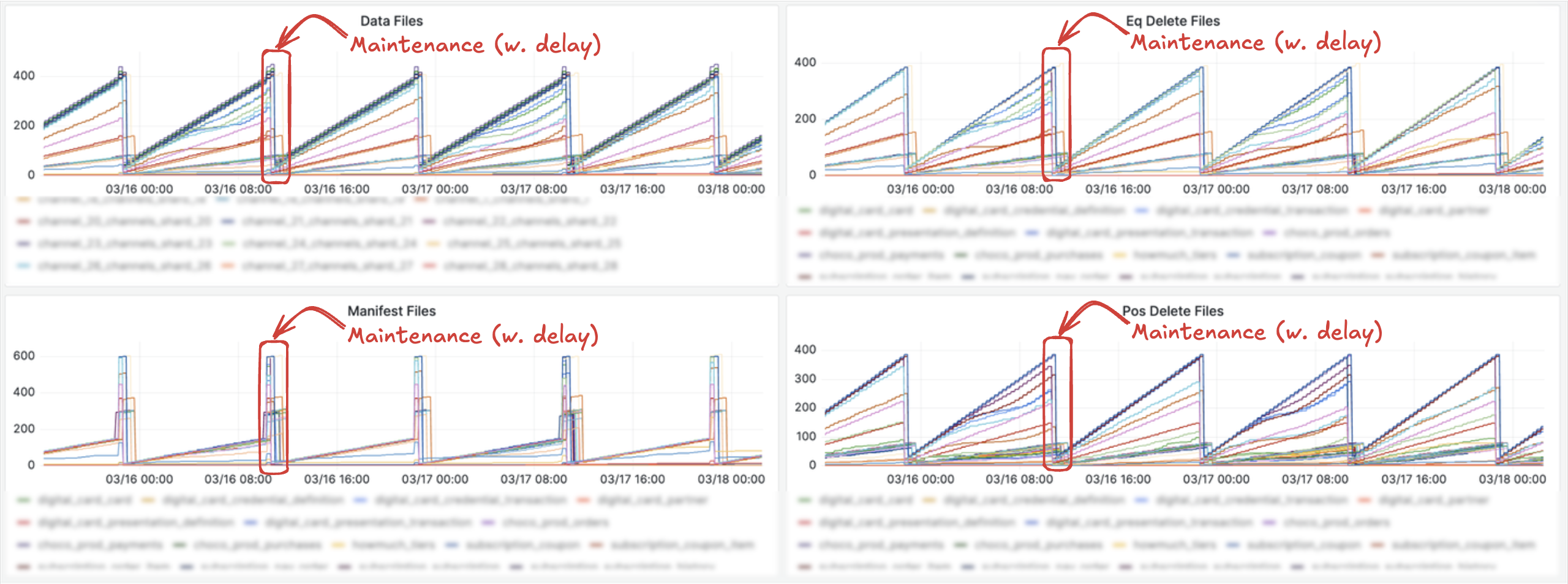
Figure 6 below illustrates the optimization process running twice daily on an Iceberg table actively loading DB logs. It also shows the increase in the number of manifest files when partial-progress.enabled is set to true. Following this, you can also see how files are subsequently deleted by the Snapshot Expiration and Delete Orphan Files processes.
For server logs, to reduce the Kafka Lag Count compared to the previous method of loading into ORC format, we ingest data using a shorter checkpoint interval. We decreased this interval from 3 minutes to 1 minute. As shown in Figure 7, this allows us to maintain a per-topic Lag Count that is at least one-third lower than before.
However, the shorter checkpoint interval results in smaller file sizes. These small files are inefficient for systems like the Hadoop File System (HDFS) and during Spark sourcing jobs. To handle this inefficiency, we configured and tested running Compaction, Snapshot Expiration, and Delete Orphan Files every hour on the partition corresponding to the previous hour.
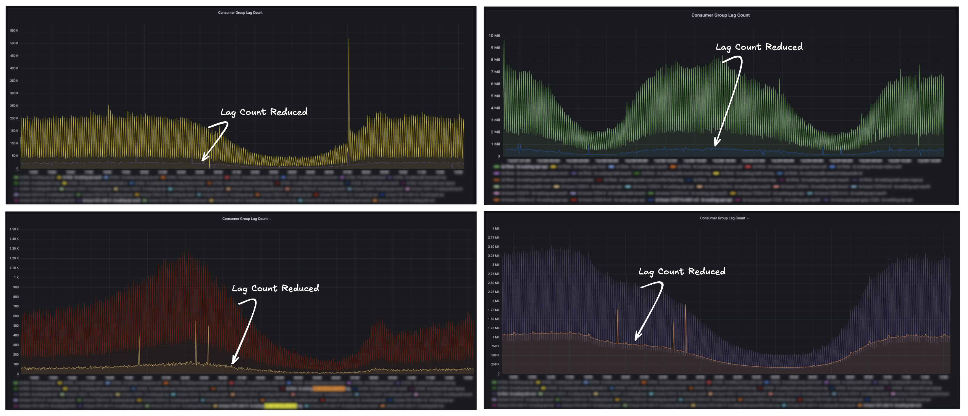
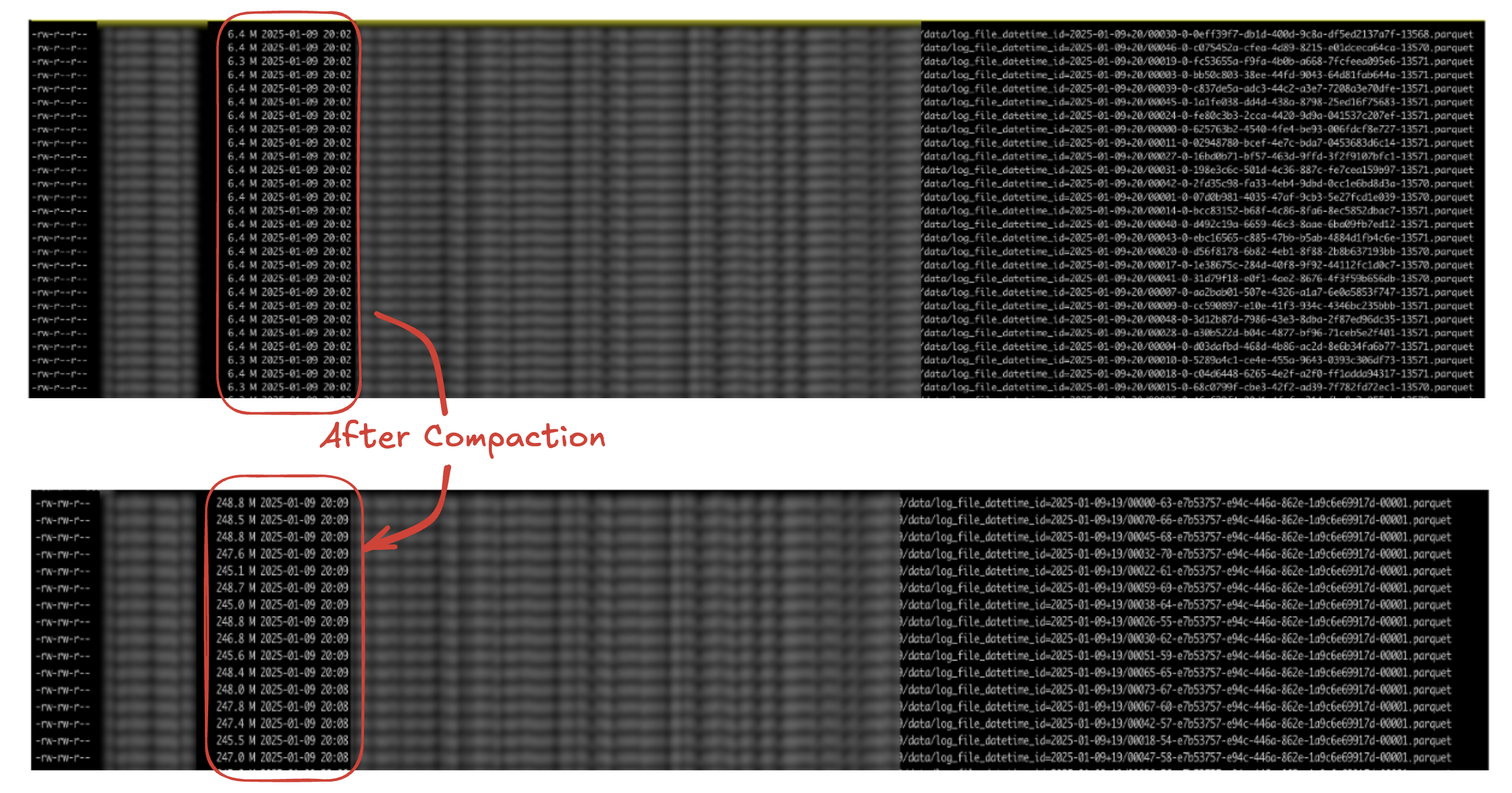
Figure 8 below shows the results of a test performed using server logs, which generate an average of 3 billion log entries per day. We can observe that small files, initially loaded at around 6 MB in size, were merged into larger files of approximately 256 MB after the optimization process, and the original small files were deleted.
Based on this, we concluded that we can shorten the checkpoint interval to lower the Lag Count while simultaneously and effectively addressing the small file problem through this optimization.
As such, DB logs and server logs require different optimization strategies because they differ in data characteristics, write mode (UPSERT vs. APPEND), and operational goals (maintaining freshness vs. high-throughput processing and lag minimization). DB logs, owing to their UPSERT nature, are managed with twice-daily all partition compaction and a relatively long retention period (20 minutes) without needing a separate delete query. In contrast, server logs, aligned with a short commit interval (1 minute), actively address the small file problem through hourly compaction of the previous hour partition and a short retention period (2 minutes).
Notably, for server logs, due to the limitations of APPEND mode, the snapshot expiration feature alone is insufficient to delete old data. This leads to a crucial difference: periodic execution of separate DELETE queries is required to enforce the actual data retention policy. These key differences in Iceberg table management and optimization strategies based on log type are summarized comprehensively in Table 10 below.
| Feature | DB Logs (Production) | Server Logs (Testing) |
|---|---|---|
| write mode | UPSERT | APPEND |
| Compaction scope | All Partitions | Previous hour partition |
| Retention (for Expire Snapshot) | 20 min | 2 min |
| Retention(for Delete Orphan Files) | 20 min | 2 min |
| Commit interval | 10 min | 1 min |
| DELETE query required | No (due to UPSERT) | Yes (due to APPEND) |
Table 10. Comparison of Iceberg Table Settings and Optimizations by Log Type
Monitoring
To operate Iceberg tables reliably and maintain optimal performance, continuously monitoring the table’s state is crucial. Specifically for Iceberg operations, it is key to verify whether small files, which directly impact query performance, are being managed effectively, if partition settings are appropriate, and if the relevant optimization jobs are running successfully. In this section, we will share the results of our tests regarding which metrics to collect and how to visualize them to achieve these operational monitoring goals.
Metrics Collection
To understand the state of Iceberg tables, metrics collection can be approached from two main perspectives. One is to monitor the state of referenced files, which directly impact query performance . The other is to track the state of all files physically present in storage, including orphan files that have not yet been deleted.
Monitoring referenced files is the most critical aspect of operating Iceberg tables. We periodically check the count, average size, and distribution across partitions of data files referenced by the latest snapshot to inspect the following:
- Whether the number of small files is increasing.
- Whether optimization jobs (like compaction) are running effectively.
- Partition appropriateness (e.g., checking for data skew towards specific partitions).
These metrics can be sufficiently obtained just by querying the metadata of the latest snapshot, utilizing Trino’s $files table or Spark SQL’s tablename.files metadata table.
Specifically, we use Trino’s $partitions table to assess the appropriateness of partition settings. This table allows us to quickly query information such as record count, data file count, and total file size for each partition. We calculate the average and Relative Standard Deviation (RSD) of the collected per-partition record counts or file sizes to verify partition suitability. Based on tests conducted on DB log tables in our production environment (specifically those using PK-based bucket transforms), the data was evenly distributed across all tables, mostly showing an RSD below 1%.
Additionally, we try to gauge the appropriate bucket size based on the table’s total file size. If the average file size per partition is too small (e.g., in the range of a few MBs), it can lead to file management overhead, prompting consideration for partition readjustment. Our approach involves setting the initial partition configuration based on the source data’s record count, and during operation, we intend to adjust the partition count based on the Iceberg table’s total file size. However, we avoid excessively increasing the bucket size, as this can paradoxically lead to the creation of small files.
Conversely, Monitoring all files is used when we need to track the count or storage usage of all files remaining in storage, or to verify how many files were removed by delete orphan files. This requires querying metadata that includes information about files referenced by expired but not-yet-deleted snapshots. Since Trino does not yet support $all_files, we currently must use Spark SQL’s tablename.all_files metadata table for this purpose.
In our operational environment, expire snapshot and delete orphan files are managed relatively reliably. Therefore, routine monitoring primarily focuses on collecting metrics for active (referenced) files based on the latest snapshot using Trino or Spark (e.g. $files, $partitions). However, we always keep the possibility of using Spark SQL’s all_files feature in mind for situations requiring an exact count of all files or detailed verification of maintenance tasks.
The metric collection frequency can be adjusted based on the table’s change frequency or importance. For CDC-integrated tables, we initially tested collection at 15-minute intervals, but we are currently testing adjustments to a collection frequency of once every 30 minutes or once per hour. We currently believe that collecting detailed per-partition metrics less frequently, perhaps once a day, will be sufficient compared to overall file count metrics.
Metrics Visualization
Visualization is a highly effective method for understanding the trends of collected metrics over time at a glance. We achieve visualization using a combination of Prometheus , Grafana , and TSCoke (an in-house time-series database provided for metric storage). Prometheus is used for storing and querying time-series data, and Grafana is used to build dashboards and various charts based on this data.
However, because Prometheus uses a pull model, fetching metrics at regular intervals, it can be incompatible with batch jobs that need to push metrics. To handle this, we incorporated the Prometheus Pushgateway. The Pushgateway acts as an intermediate gateway, allowing batch jobs to send collected metrics via HTTP requests. When a batch job collects and calculates metrics and sends them to the Pushgateway via a REST API, Prometheus then scrapes these metrics from the Pushgateway according to its configured interval.
When using the Pushgateway, the following settings and precautions should be noted. First, ensure the honor_labels option is set to true in the Prometheus scrape_config . This prevents Prometheus from altering the unique labels generated by the batch job (e.g., metric_name{label1="value1", label2="value2"}) to avoid potential label conflicts, ensuring your intended labels are preserved.
Second, it is recommended to explicitly distinguish metric groups by including identifying information in the URL path . If labels are only included in the metric payload without differentiating groups in the URL path, identical metrics from different tables might be treated as a single group, potentially resulting in the last transmitted metric overwriting previous ones. To solve this, grouping information should be explicitly specified in the REST API’s URL path, such as $PUSHGATEWAY_URL/metrics/job/$namespace/table/$table.
Finally, the POST HTTP method is recommended for sending metrics. The PUT method completely replaces all existing metrics within that URL path group with the newly sent metrics, which can lead to unintentional metric loss. In contrast, using POST only updates the value of the metric with the same name and labels, allowing you to safely maintain and update existing metrics without affecting others in the group.
The metrics collected and stored this way are visualized through Grafana dashboards, like the one shown earlier in Figure 6. Through these dashboards, we monitor the trends over time for metrics such as the total number of data files, delete files, and manifest files. We also verify that optimization jobs are effectively preventing the accumulation of small files, keeping their count below a certain level.
Conclusion
I sincerely thank all readers of this article.
In this article, we shared our journey of efficiently managing DB logs and server logs, each with distinct characteristics, using Iceberg tables. For DB logs, we covered our stable operational experience using CDC, UPSERT mode, and bucket transform partitioning. For server logs, we discussed the optimization process involving APPEND mode, processing time-based identity transform partitioning, and testing zstd compression levels. Additionally, we examined optimization strategies for stable operation, such as compaction and snapshot management, along with monitoring methods. However, regarding the server logs, we wish we could have also shared our experience applying these strategies in a production environment, beyond the test results discussed.
Through this process, we learned that the structure and detailed settings of the pipeline can vary significantly depending on the purpose of using Iceberg tables and the data consumption patterns. If any readers are planning similar tasks, we recommend first clearly defining the objectives for loading data into Iceberg tables and how the data will be consumed. Then, design the pipeline structure and specific configurations accordingly.
Furthermore, although not included in the main body of the text for flow reasons, issues such as the deletion of metadata files can occasionally occur during operations, causing the Iceberg table integration to break. In such cases, one typically uses Spark SQL with DROP TABLE to remove only the table registration while preserving the physical files. Then, the table is re-registered using the register_table(table => ‘’, metadata_file => ‘’) procedure based on a past metadata file. Afterward, recovery is possible by reprocessing data from that past point in time, accepting some data duplication. Also, please keep this in mind that for such recovery scenarios, it’s important to carefully tune Flink’s checkpoint interval and the maximum number of retained metadata files (default: 100), as these settings determine the furthest point in the past to which you can recover.
Finally, I would like to express my gratitude to our team that supported this work.