Optimal VM Density Testing for Efficient VMWare Infrastructure Operation

이 글은 < 효율적인 VMWare 인프라 운영을 위한 최적의 VM 집적도 테스트 >를 영어로 작성한 문서입니다.

다른 번역본 보기:

🇰🇷 한국어: https://tech.kakao.com/posts/634

🇯🇵 日本語: https://tech.kakao.com/posts/637

🇺🇸🇬🇧 English: https://tech.kakao.com/posts/638

---

1. Beginning

With the advancement of virtualization technology, it has become commonplace to run multiple VMs (Virtual Machines) on a single PM (Physical Machine). VMWare is a leading provider of such virtualization technology, and Kakao is operating a sizable VMWare infrastructure.

When operating such a VM infrastructure, the question of ‘how many VMs to run on a PM’, or VM density, becomes a concern. Everyone knows that as the number of VMs running on a single PM increases, the performance of the VMs decreases due to increased contention for limited PM resources. However, it’s not easy to give a clear answer when it comes to specifics like ‘how much performance degradation occurs’ or ‘at what number of VMs does performance degrade dramatically’.

In fact, it is difficult to define these in a generalized way because they depend on the operating environment, such as the specifications of the PM and the resource usage of the VM. However, I thought that if we limit the scope of the test to the conditions that correspond to the current operating environment, we can derive the optimal VM density that can serve as a reference at least for the current operating environment. Also, I thought that having an overall understanding of VM density would be helpful even if the operating environment changes in the future.

In this article, I would like to share my experience with testing to find the optimal VM density from a CPU perspective for operating a VMWare infrastructure efficiently.

2. Test Introduction

The purpose of this test is to determine the optimal VM density from a CPU perspective, that is, the maximum number of VMs that can be accommodated on a single PM without degrading the CPU performance of the VMs. In addition to CPU, other factors that determine optimal VM density include memory and disk, but for this test, I focused on CPU.

1) Basic Idea

The basic idea of the test is to progressively increase the number of VMs on a single PM, measure the CPU performance of VMs, and find the number of VMs where the CPU performance of the VM starts to degrade below the threshold.

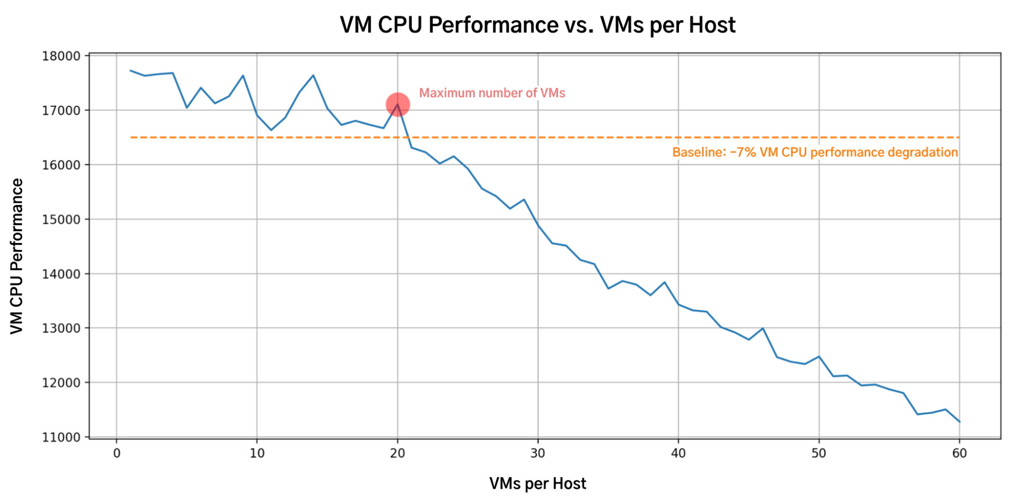
For example, if the VM CPU performance degradation threshold is set to 7% for service stability, as shown in the figure above, if VM performance begins to degrade beyond this threshold once the number of VMs simultaneously running on a single PM exceeds 20, then the maximum number of VMs that can be accommodated by the PM can be said to be 20.

An important consideration is how to measure the CPU performance of VMs that are affected by resource contention with other VMs. In this test, I ran the benchmark program on all VMs deployed in PM at the same time and averaged the results. This means that the benchmark program not only measures the CPU performance of the VM itself, but also acts as a load that causes resource contention for other VMs.

2) CPU Usage of VM

How much CPU load to allocate to VMs is also important, as the CPU usage of VMs determines the maximum number of VMs that can be accommodated on a single PM.

Actually, in operating environments where the average CPU usage of VMs is not high, it is common to run many VMs relative to the number of physical cores in the PM (a.k.a. CPU Overcommit) in order to increase the resource utilization of the PM. Therefore, in order to obtain results that could be referenced during practical operation, tests were conducted by increasing the CPU usage of the VM from 10% to 100% in increments of 10%.

To simulate a situation where all VMs in a PM are using a certain percentage of CPU, the benchmark program was run with the maximum CPU usage of the VMs limited. Since the benchmark programs used in the tests are designed to use the maximum available CPU resources, setting a CPU usage limit on the VM and running these benchmark programs allows for the adjustment of the VM’s CPU usage to the desired level.

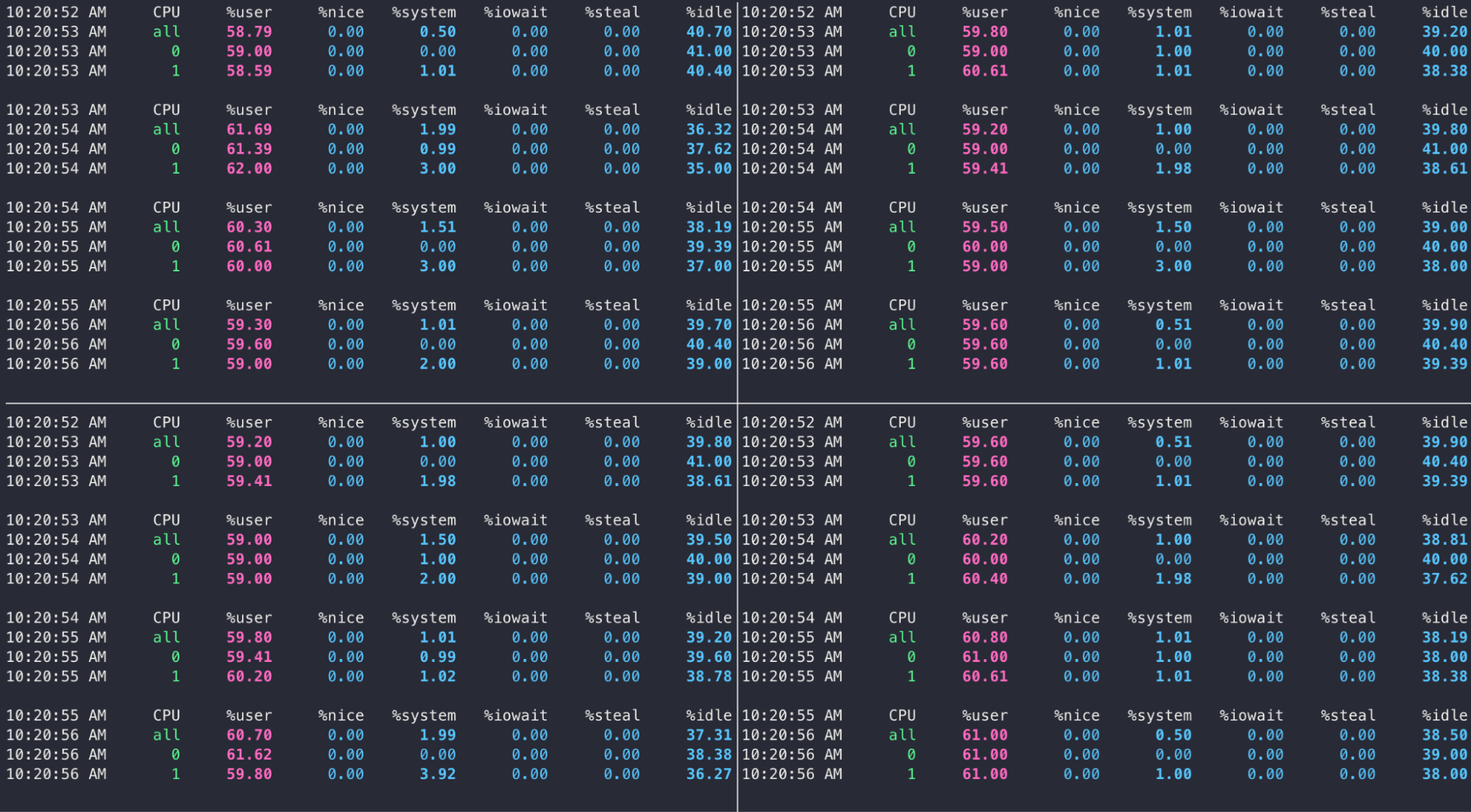
Naturally, running a benchmark program with the VM’s CPU usage limited will result in a lower score than if the CPU usage was 100%. However, the subject we are trying to compare is not the performance when the CPU usage of the VM is different, but the performance when the number of VMs is different while the CPU usage of the VM is the same. Therefore, it is not a problem that the benchmark score is measured lower in proportion to the CPU usage of the VM.

3) Flavor of VM

The optimal VM density can vary depending on the number of CPUs (vCPUs) in a VM, or in other words, the flavor of the VM. Because PM has limited CPU resources, the number of VMs you can accommodate depends on how much CPU resources to allocate per VM.

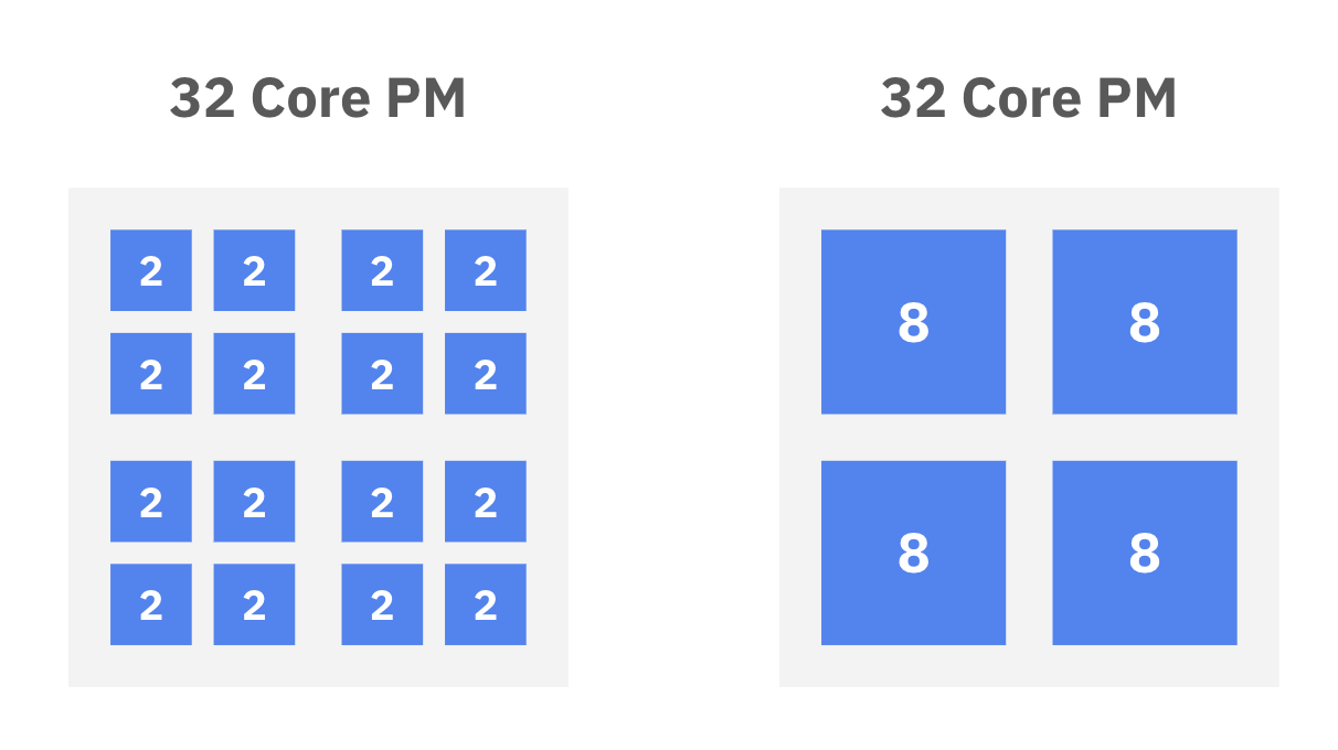
As a simple example, if there is a PM with 32 cores (pCPUs) as shown above, and the VMs are deployed so that the total number of vCPUs in the VMs equals the number of cores in the PM, sixteen 2 vCPU VMs might be deployed, and four 8 vCPU VMs might be deployed.

To determine the optimal VM density for each flavor, tests were run for three flavors: 2 vCPU / 4 vCPU / 8 vCPU to see how many VMs of each flavor could be accommodated in a single PM. While it is possible to run VMs of different flavors on a single PM, this test assumes that all VMs in the PM are of the same flavor.

4) CPU specifications of PM

The CPU specifications of the PM are also an important factor that affects optimal VM density. The optimal VM density depends on the number of cores, cache memory size, and more.

In particular, the number of cores directly affects the maximum number of VMs that can be accommodated.

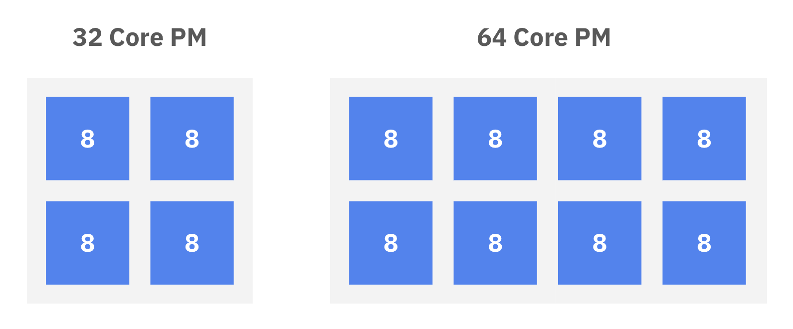
As a simple example, if a PM has twice as many cores, as shown in the figure above, it can be expected to accommodate twice as many VMs.

Two CPUs were used in this test: an Intel Xeon Silver 4410Y and an Intel Xeon Silver 4214. Although the core count is the same between the two CPUs, there may be differences in VM density due to differences in CPU generation. To verify this, the CPU specifications of the PM were taken into account as a variable in this test.

5) Test Procedure

Based on the above, tests were conducted to determine the optimal VM density for each condition.

Test Environment

PM (CPU specifications and hypervisor version)

	Processor	Sockets	Cores per Socket	Threads per Socket	Total Threads	Hyper-Threading	Base Frequency	Turbo Frequency	Cache Size	Hypervisor Version
Sapphire Rapids CPU PM(Vendor A)	Intel Xeon Silver 4410Y	2	12	24	48	Enabled	2.00GHz	3.90GHz	30MB	VMWare ESXi 8.0.2
Sapphire Rapids CPU PM(Vendor B)	Intel Xeon Silver 4410Y	2	12	24	48	Enabled	2.00GHz	3.90GHz	30MB	VMWare ESXi 8.0.2
Cascade Lake CPU PM	Intel Xeon Silver 4214	2	12	24	48	Enabled	2.20GHz	3.20GHz	16.5MB	VMWare ESXi 7.0.2

For the Sapphire Rapids CPU PMs, the same tests were conducted on PMs from two vendors with identical specifications for cross-vendor comparisons.

Flavor of VM

• 2 vCPU 4GB MEM

• 4 vCPU 8GB MEM

• 8 vCPU 16GB MEM

CPU Usage of VMs

• From 10% to 100%, in 10% increments

Number of VMs

• From 1 to 60, in increments of 1

Benchmark Programs

• CoreMark

• stress-ng

Test Method

Measure the CPU performance of the VMs by varying the number of VMs and the CPU usage of the VMs for each combination of PM and VM flavor.

The sequence of tests is as follows.

1. Deploy N VMs of a specific flavor, on a specific PM, in increments of 1 to 60 VMs.

2. Set CPU usage limit for N VMs from 10% to 100% in 10% increments.

3. Run a benchmark program on N VMs simultaneously.

4. Aggregate the results of the benchmark for each CPU usage of N VMs and calculate the average.

In other words, for each combination of PM and VM flavor, the following nested for loop is executed, measuring the CPU performance of the VMs for a total of 600 cases for each of the number of VMs and the CPU usage of the VMs.

for N in range(1, 60, 1): # Increment the number of VMs(N) by 1 from 1 to 60
	# Deploy N VMs to PM
	for M in range(10, 100, 10): # ​​Increase the CPU usage limit(M) for VMs from 10% to 100% in 10% increments
		# Run a benchmark on N VMs simultaneously with a CPU usage limit of M%
		# Aggregate benchmark results for each VM

6) Test Results

After conducting the test, VM CPU performance results by the number of VMs and CPU usage of VMs can be obtained, for each combination of PM and VM flavor.

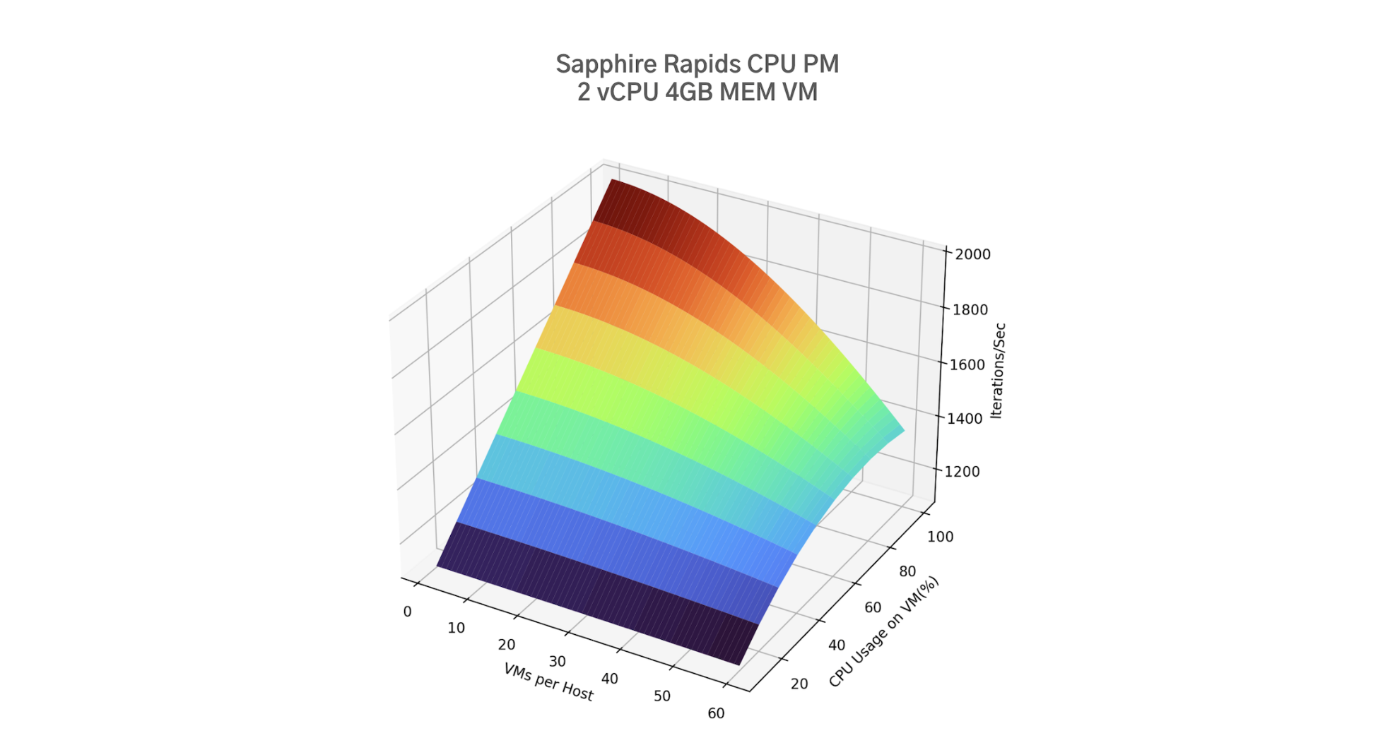
To illustrate the results in a way that shows all the factors in the best possible light, for each combination of PM and VM flavor, a graph can be plotted with the number of VMs on the x-axis, the CPU usage of the VMs on the y-axis, and the average of the benchmark scores on the z-axis, as shown above.

The graph above was plotted before running the test, anticipating what the overall results would be. It was expected that the CPU performance of VMs would decrease as more VMs, using more CPUs, increase competition for limited CPU resources.

How the results are visualized can vary depending on the purpose, but essentially, the results of this test provide the point at which a VM’s CPU performance begins to degrade below a threshold for each condition - the optimal VM density.

3. Changes in CPU performance of VMs as the number of VMs increases

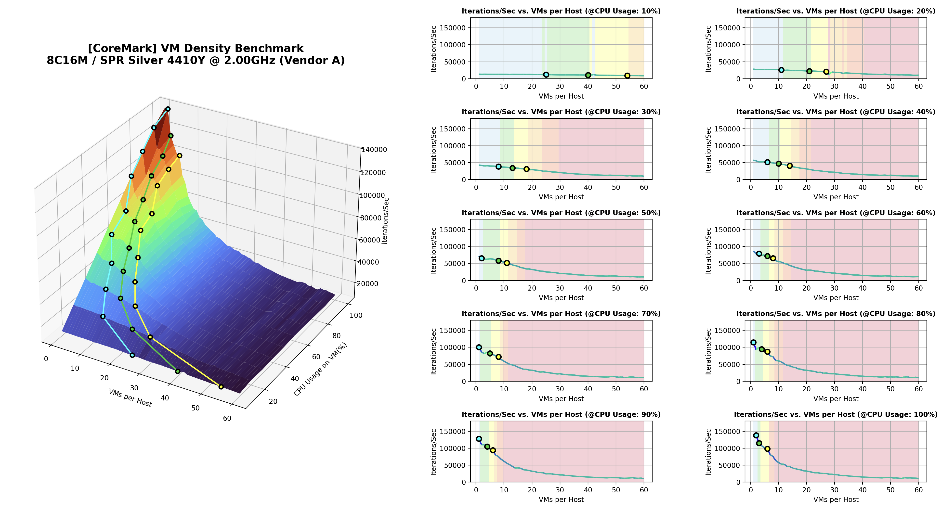
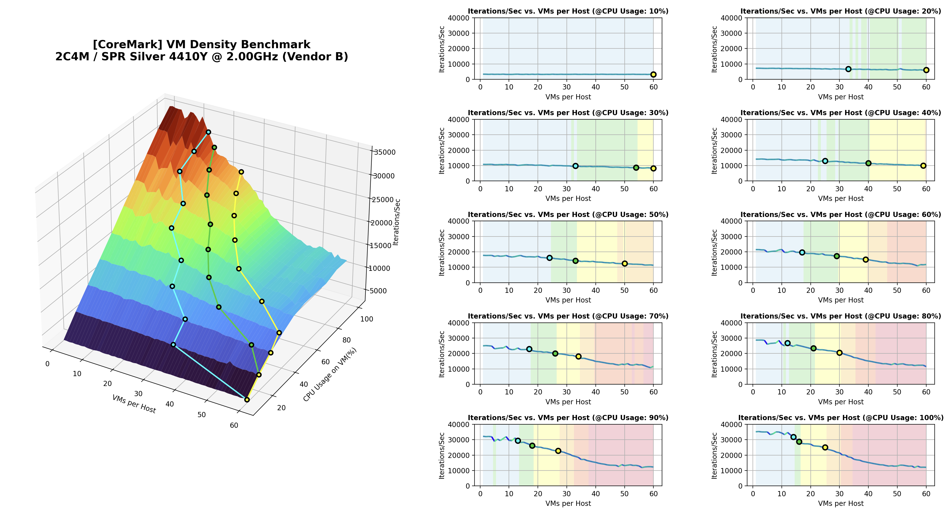
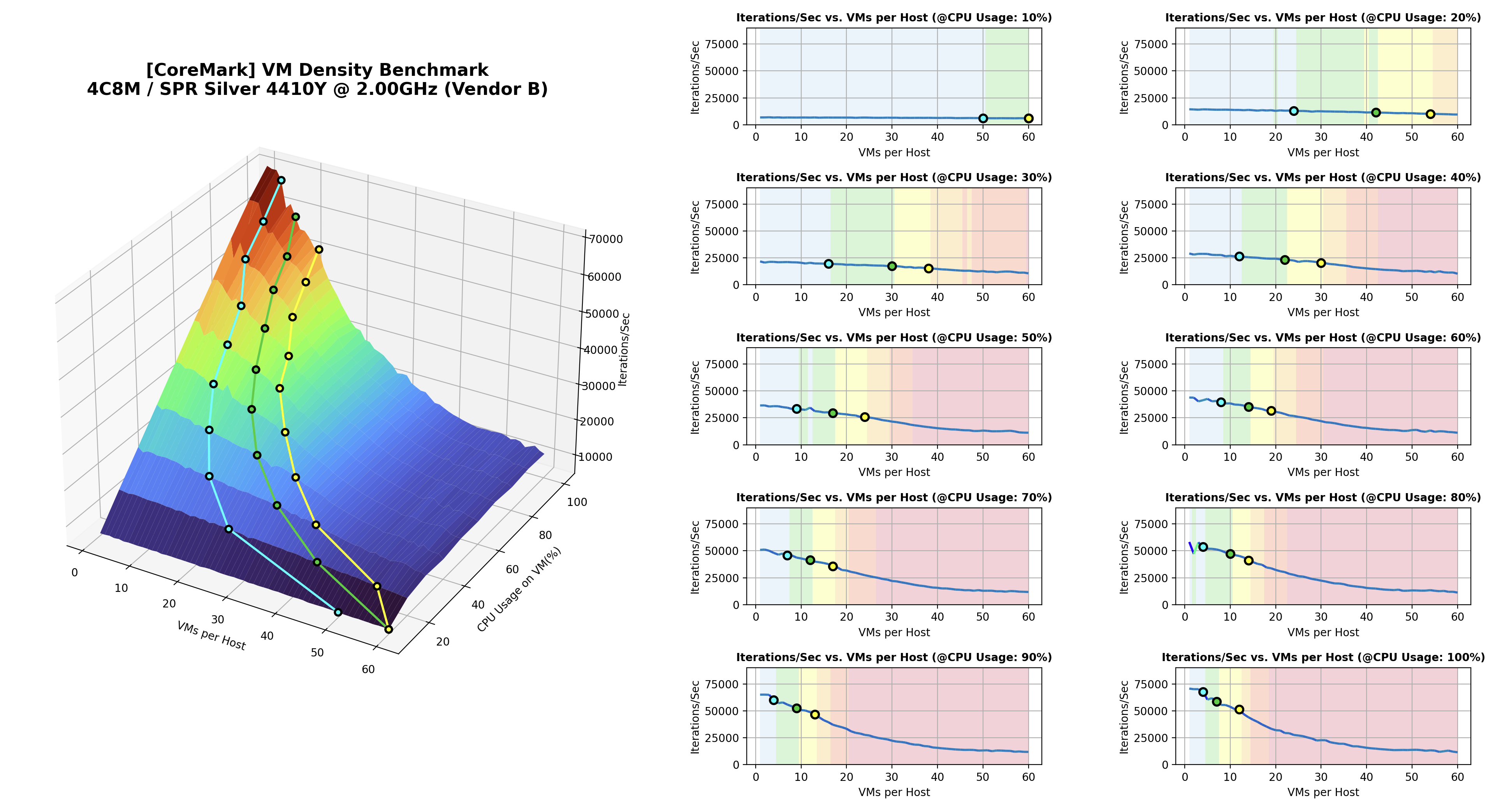
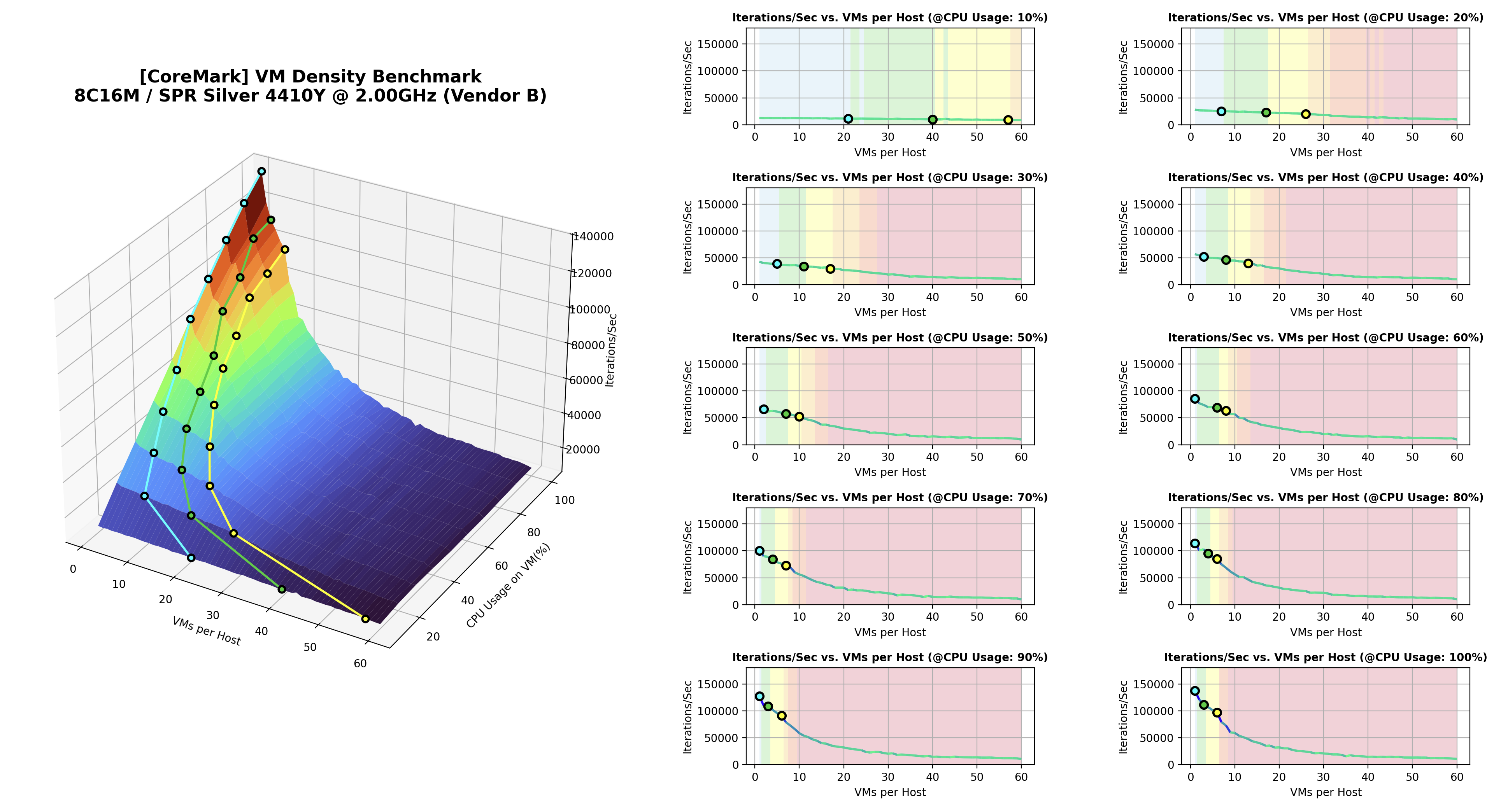
	SPR Silver 4410Y @ 2.00GHz (Vendor A)	SPR Silver 4410Y @ 2.00GHz (Vendor B)	Cascade Silver 4214 @ 2.20GHz
2 vCPU 4GB MEM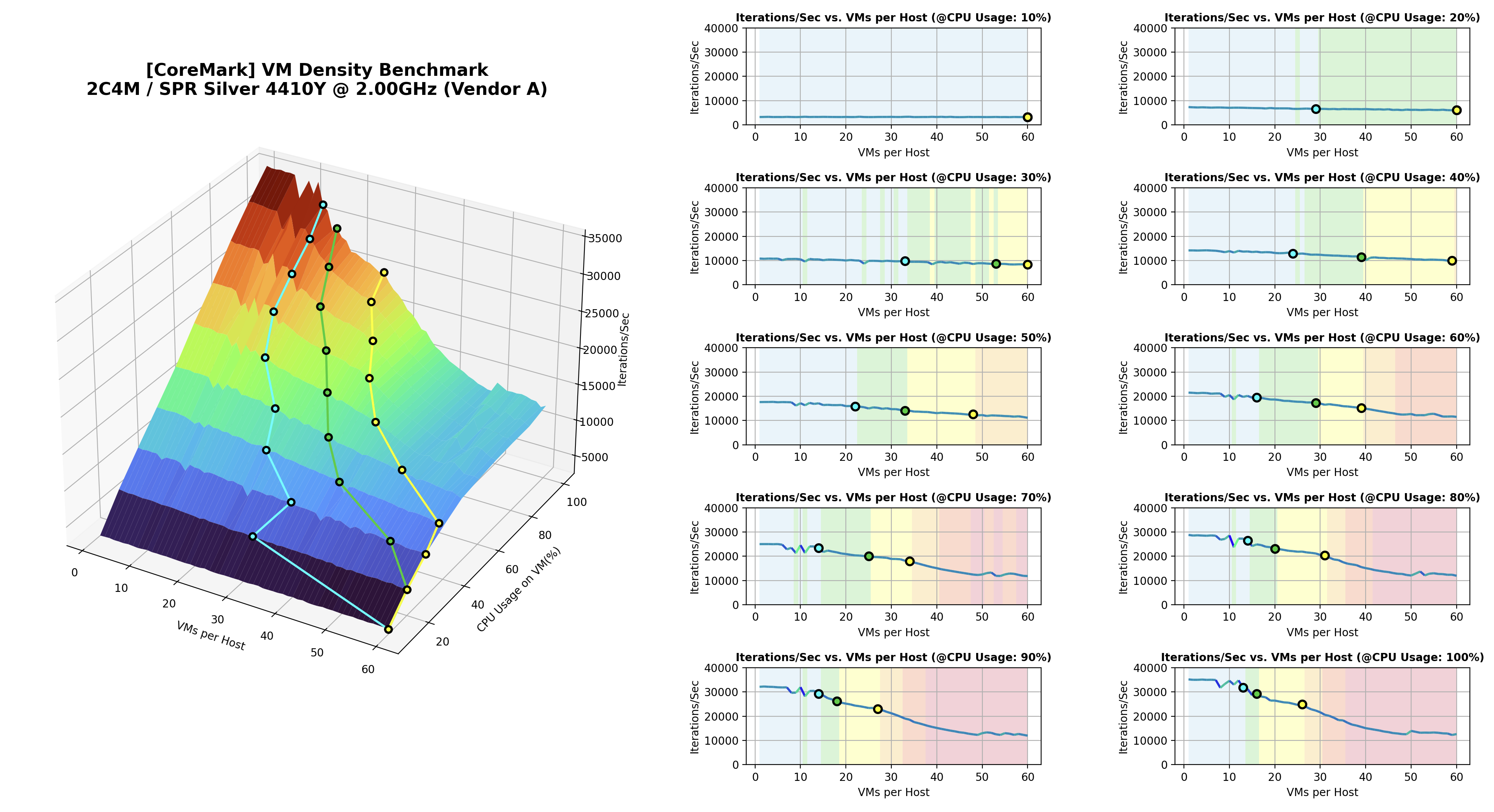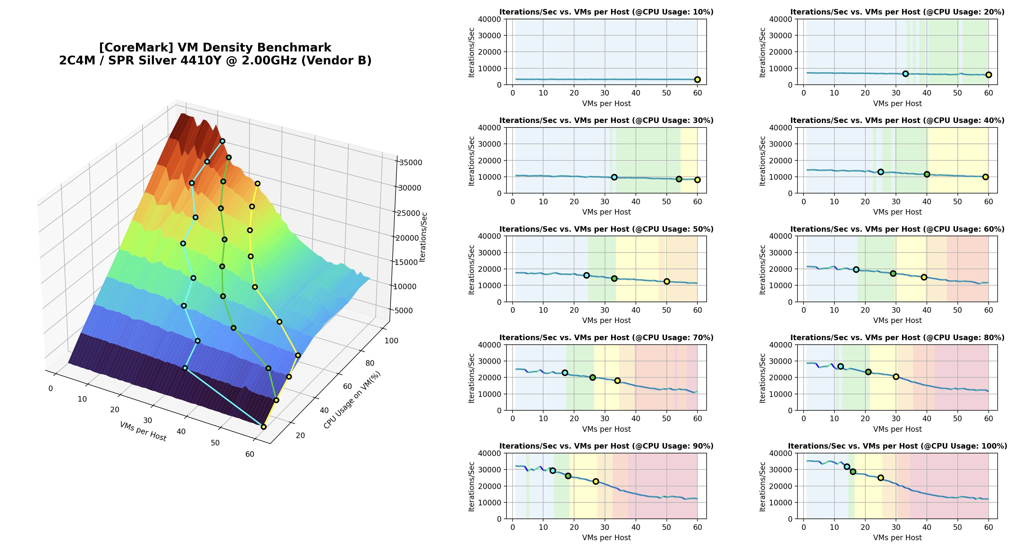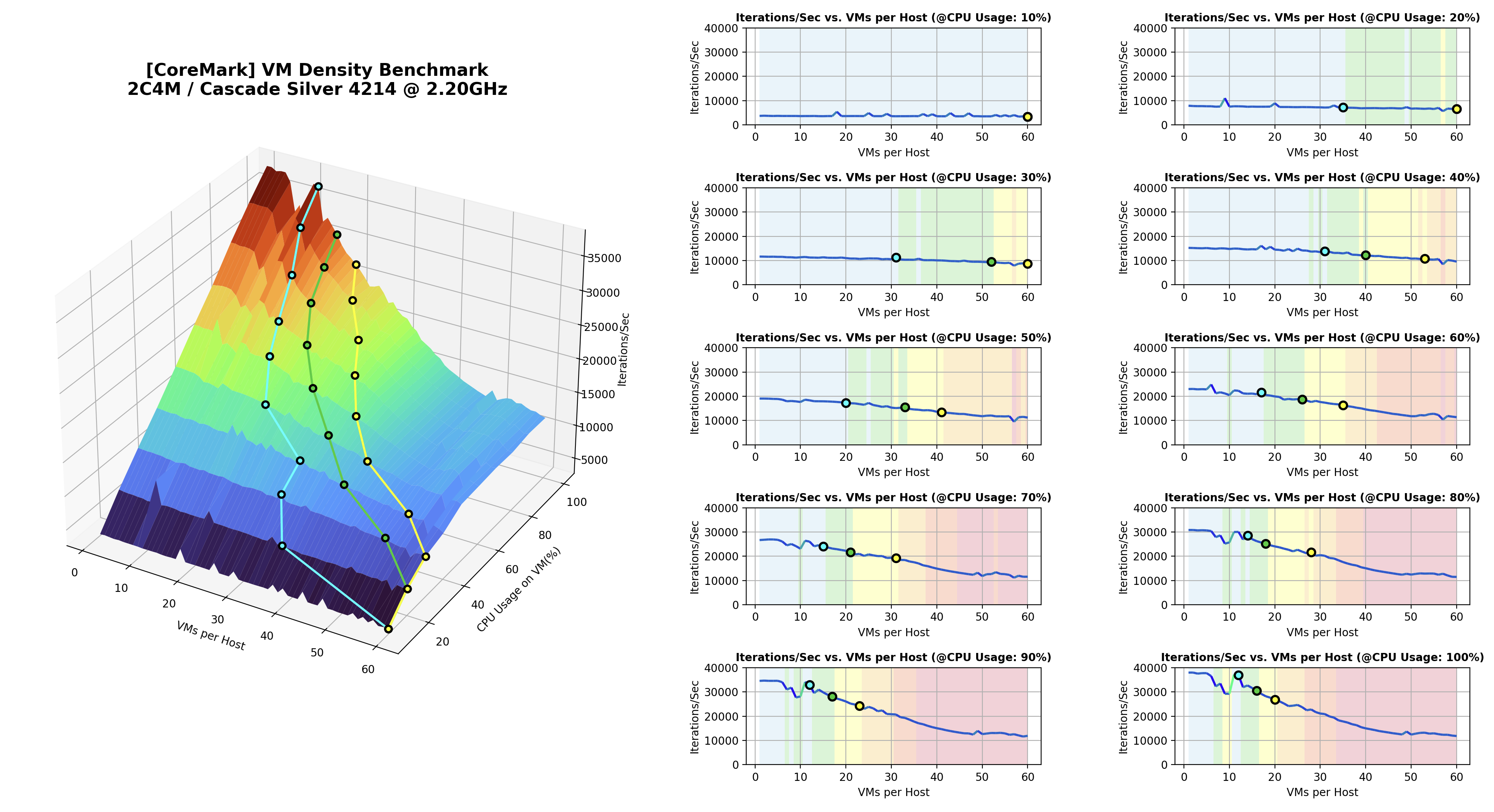
4 vCPU 8GB MEM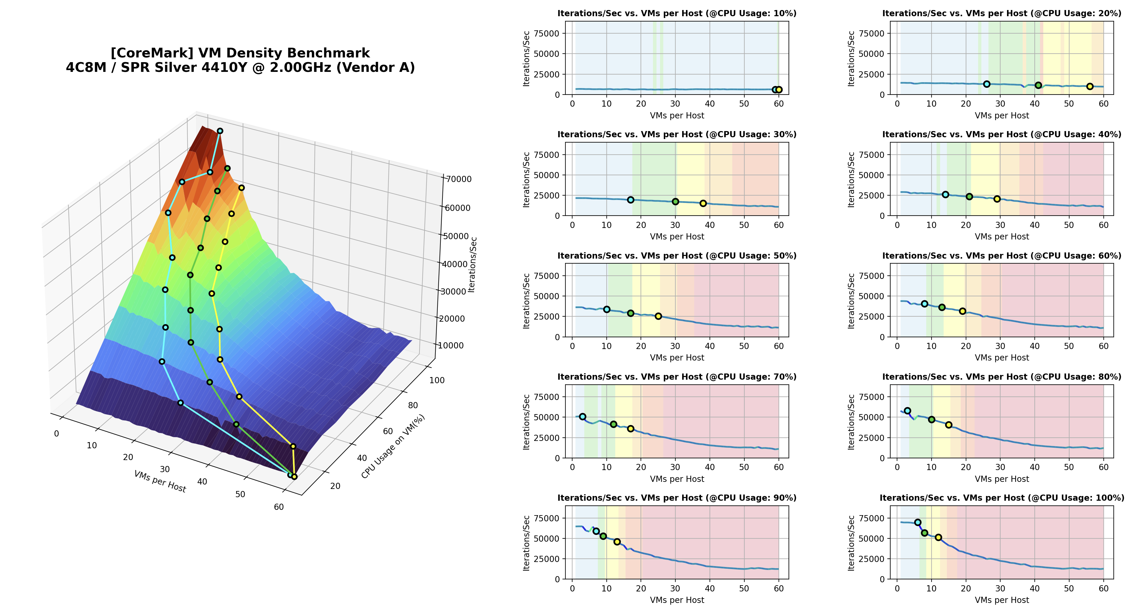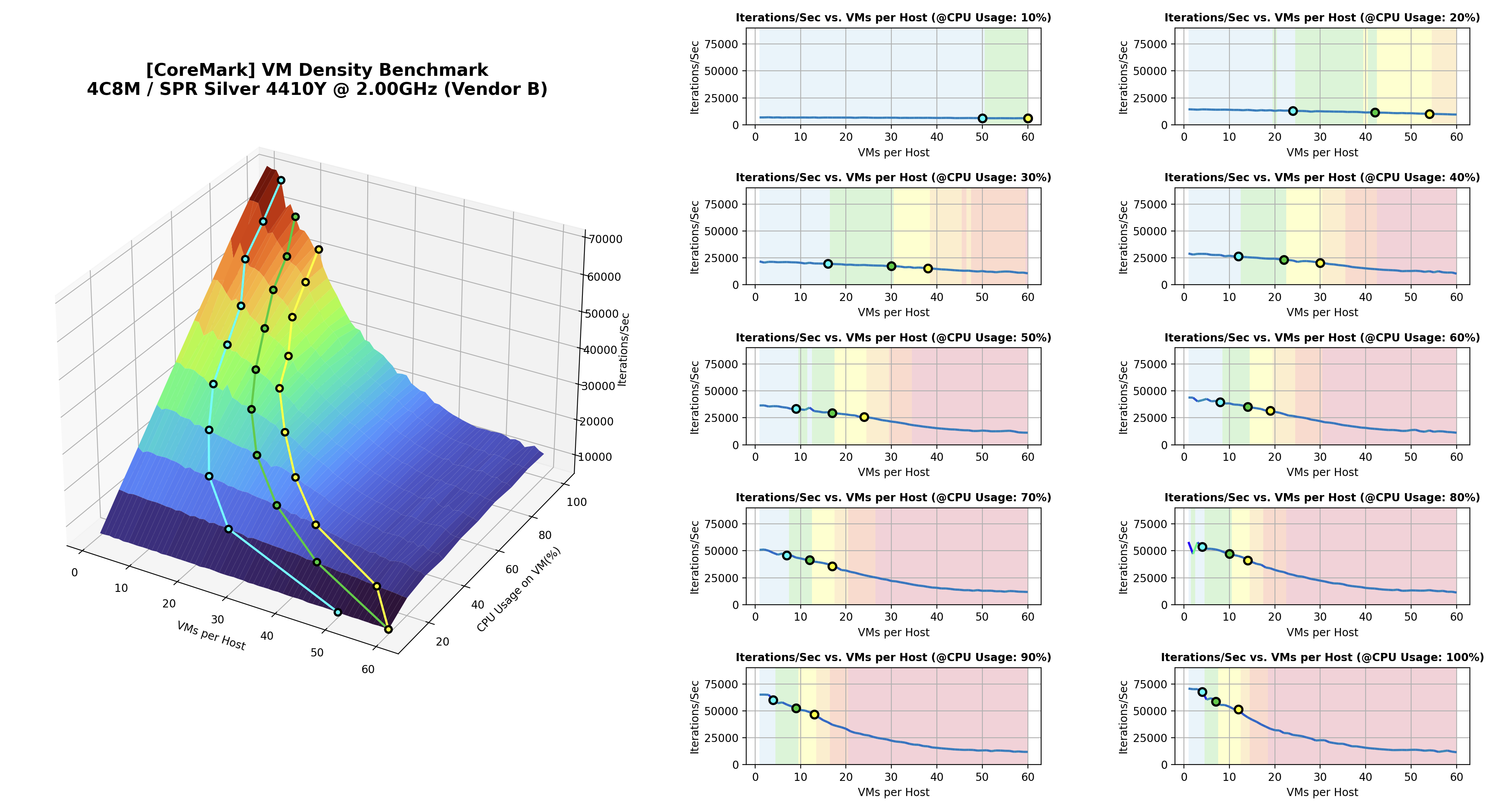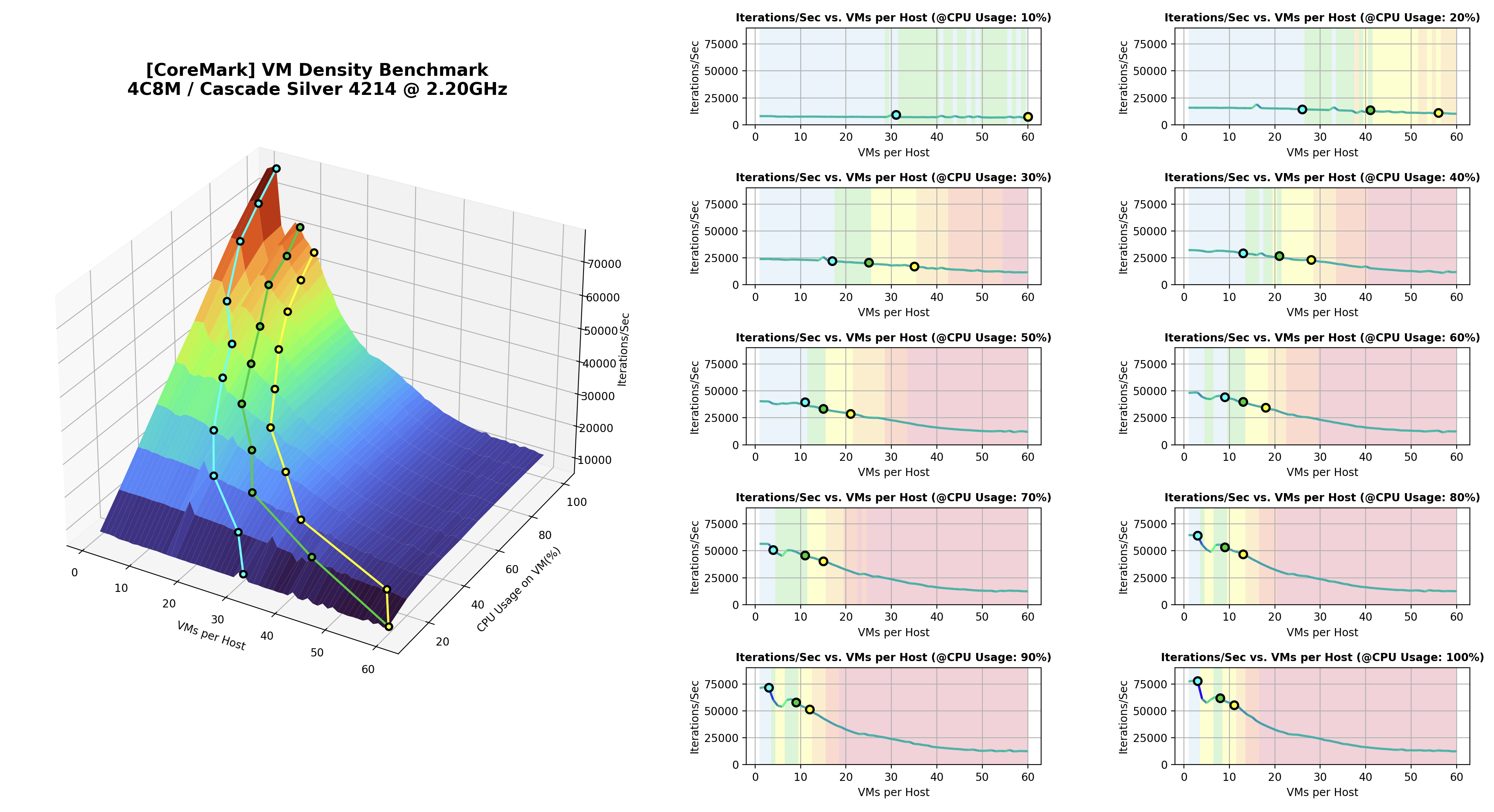
8 vCPU 16GB MEM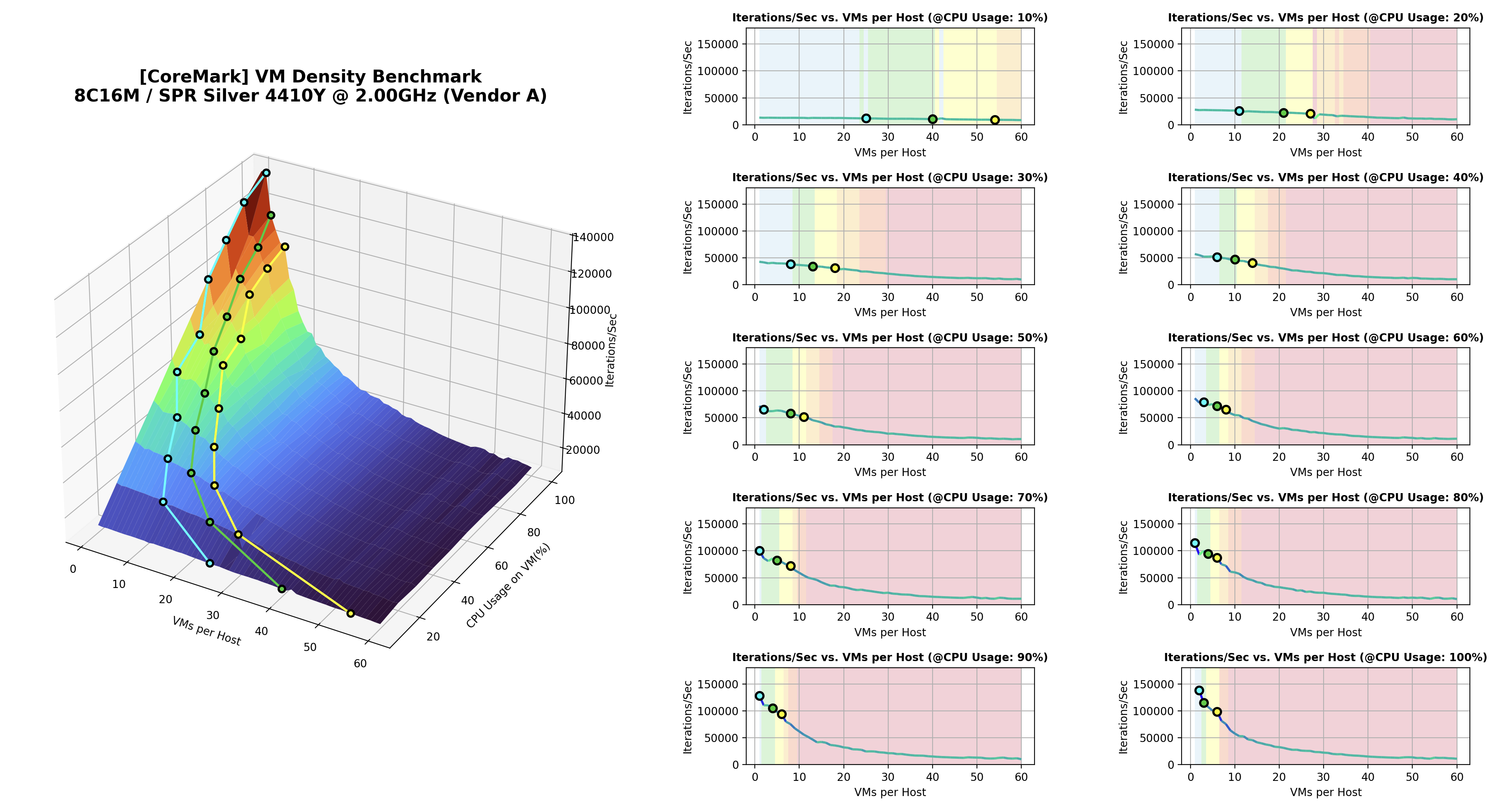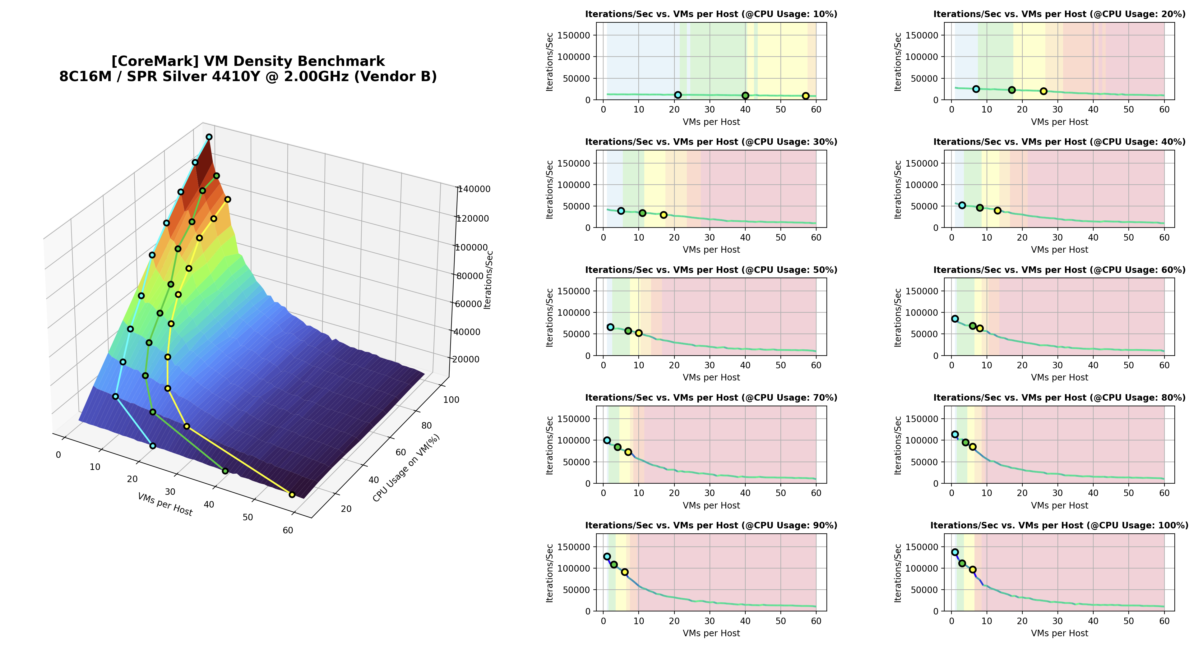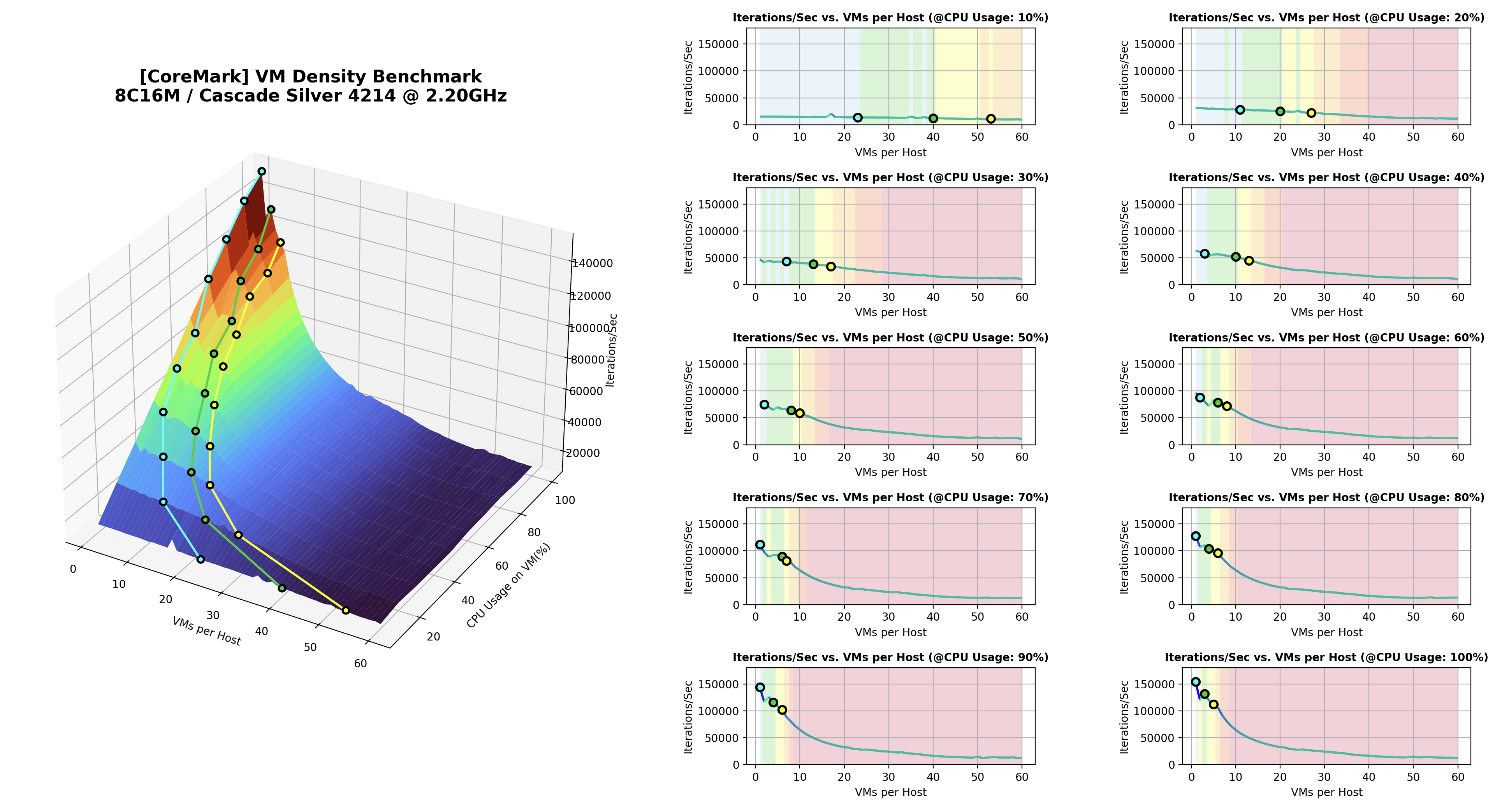

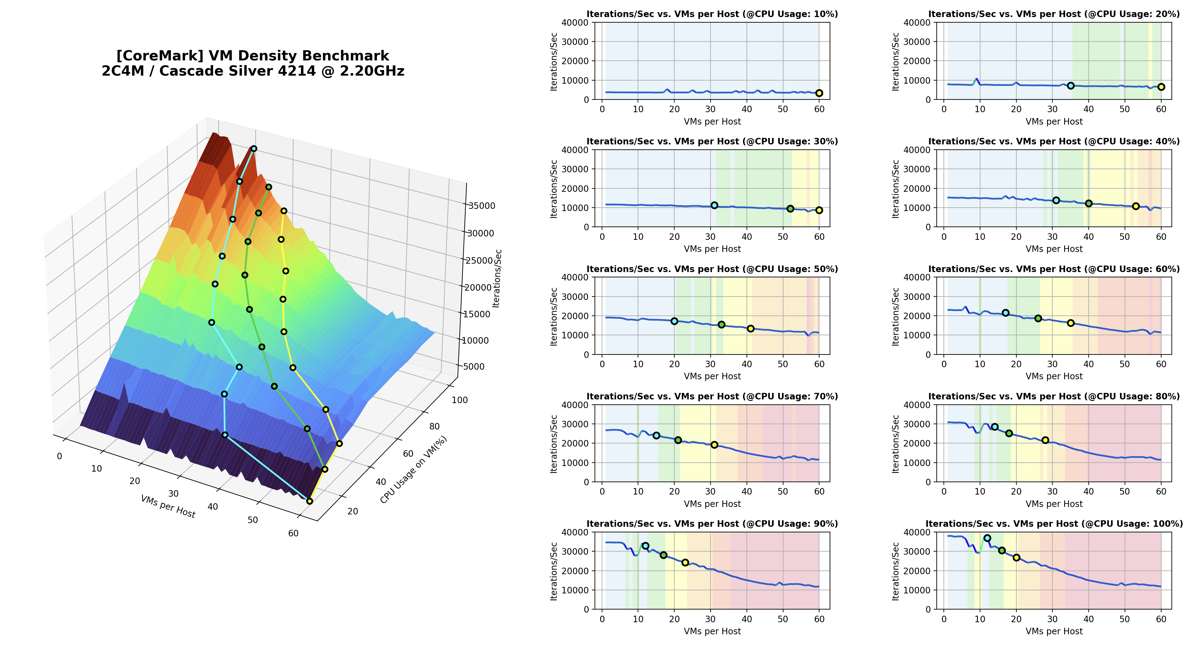
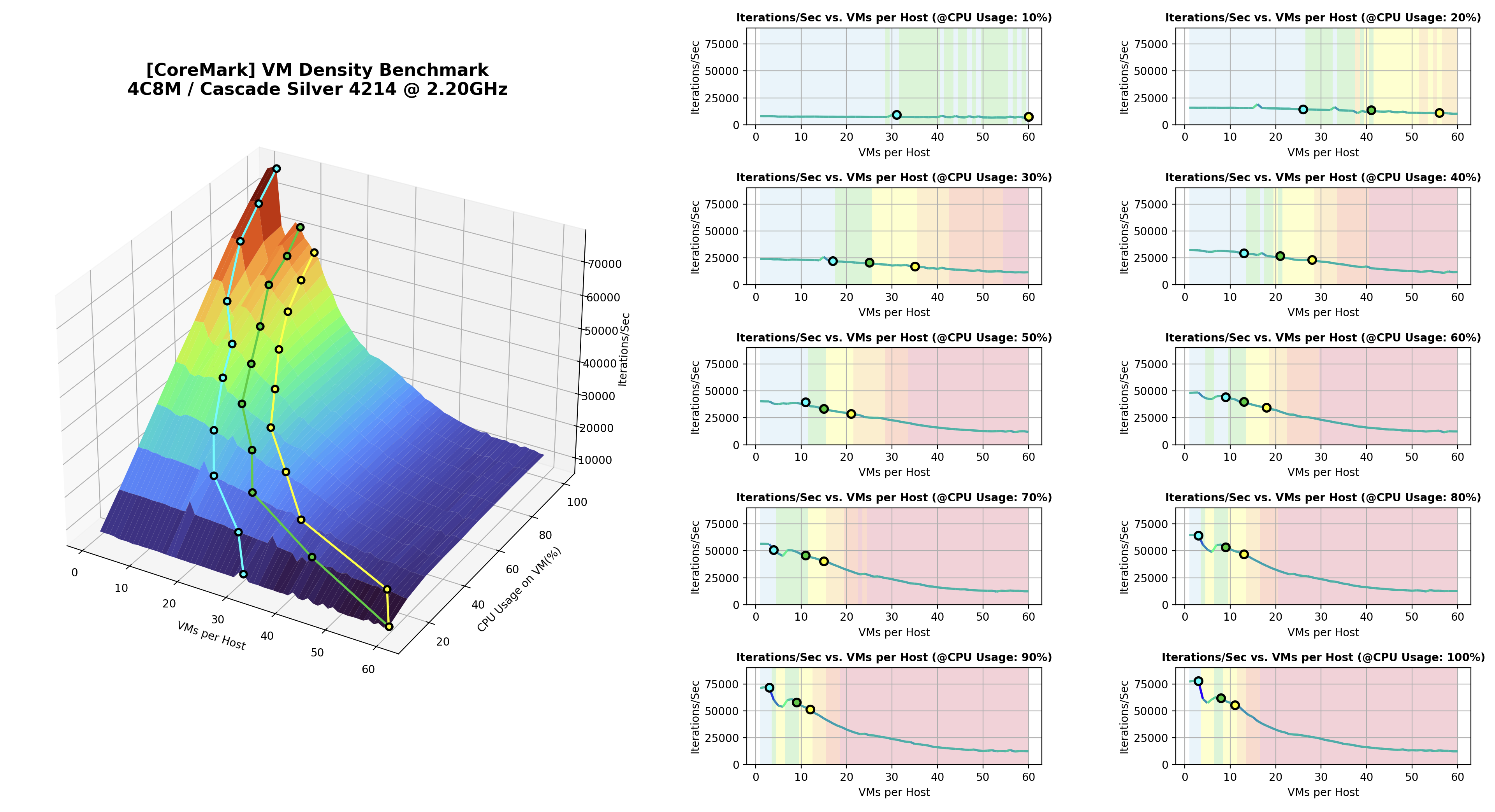
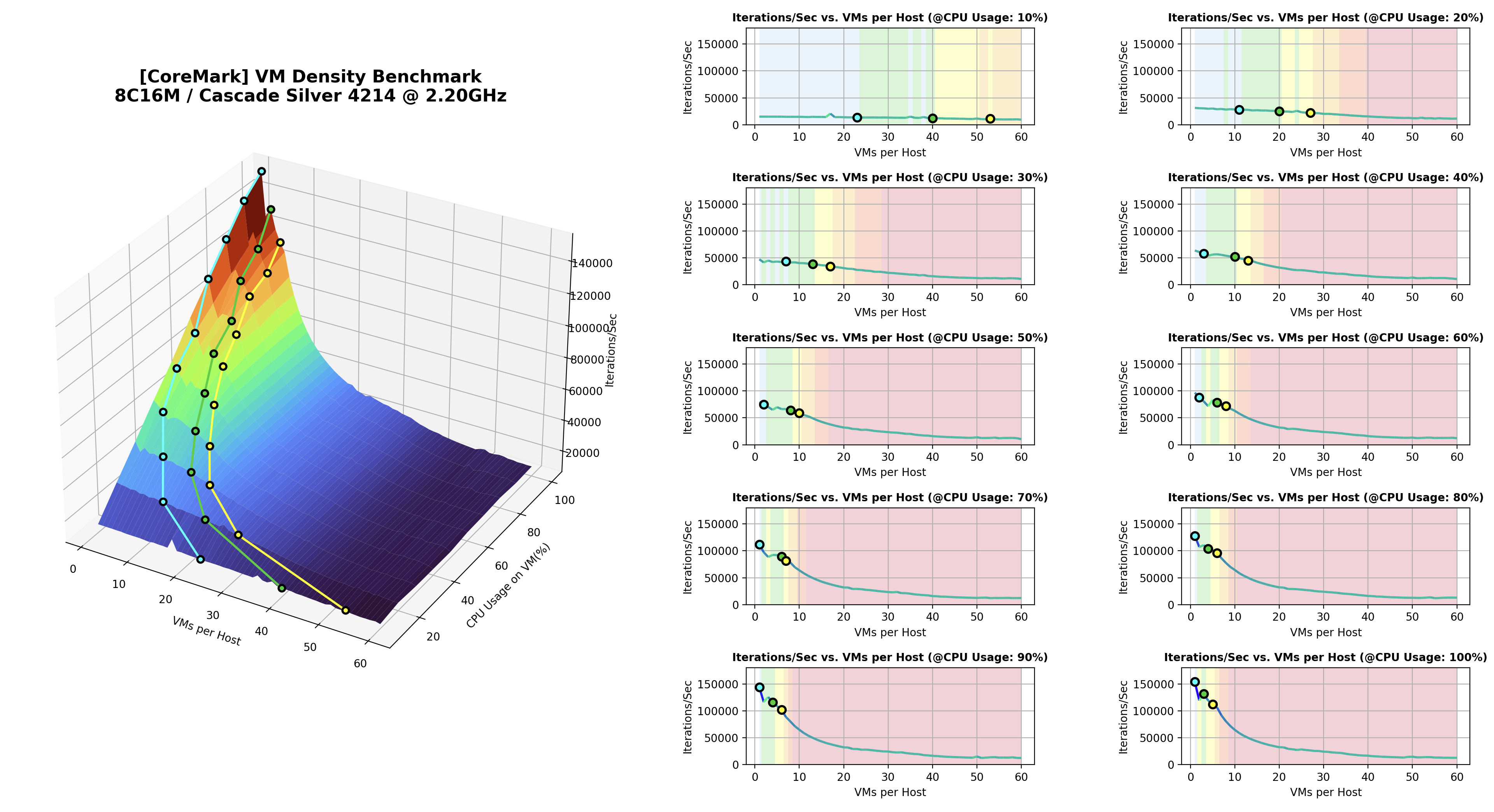
< Results for all combinations of PM specifications and VM flavor >

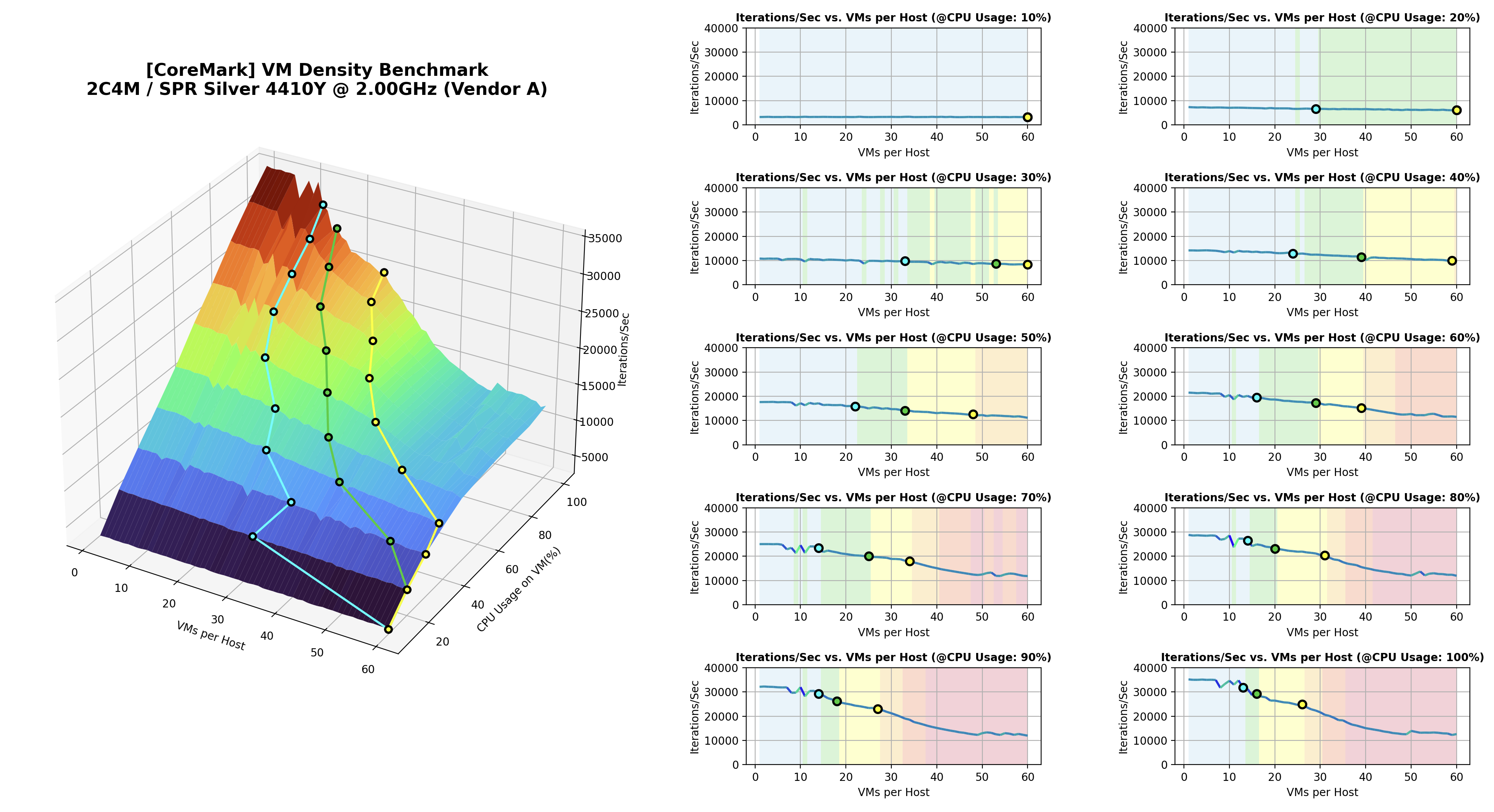
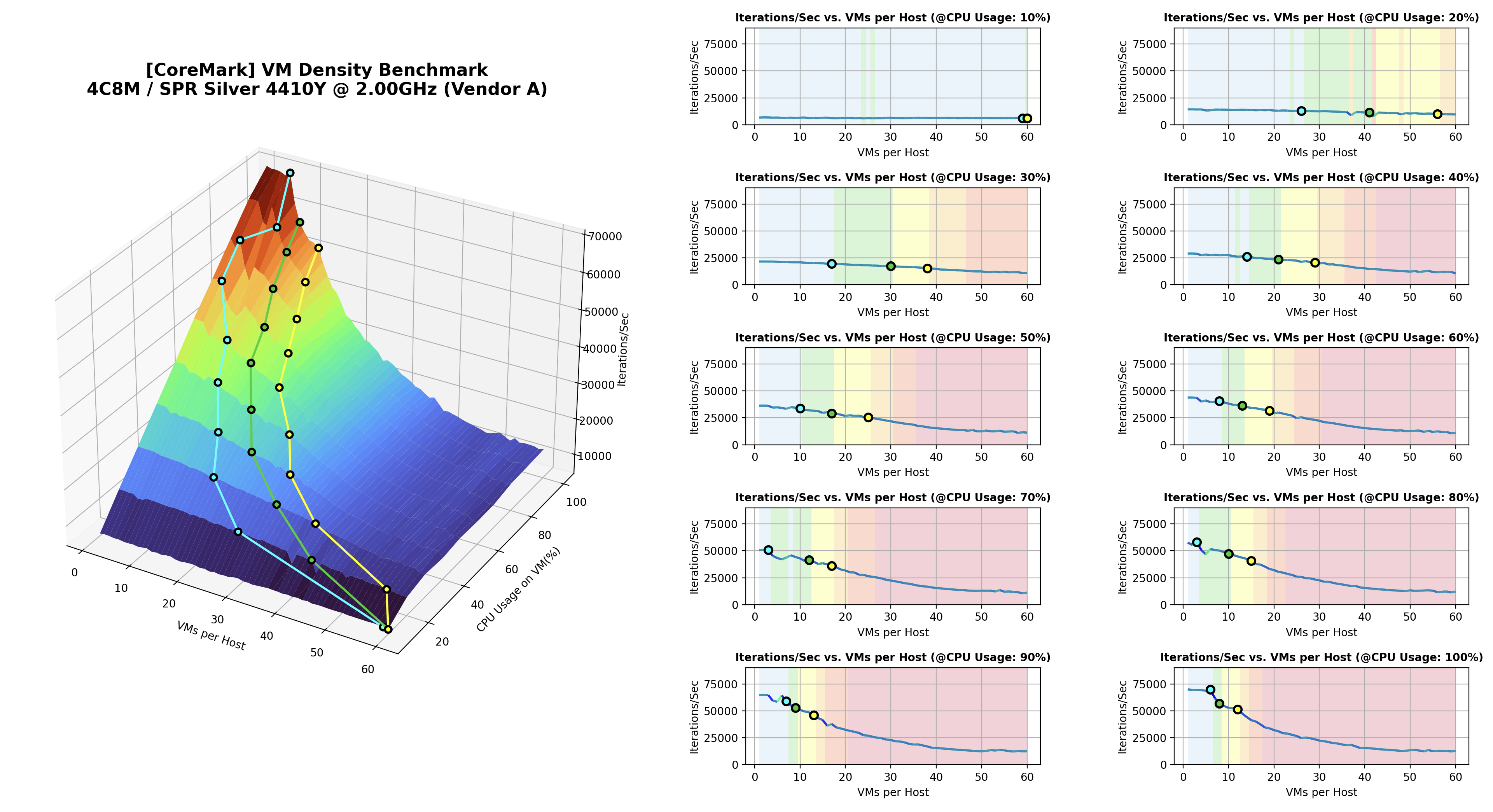
1) Data Overview

The graphs above show the change in the CPU performance of VMs as the number of VMs increases by the CPU specifications of the PM, the flavor of the VM, and the CPU usage of the VM. The purpose is to see an overall picture of how the VM’s CPU performance decreases under each condition.

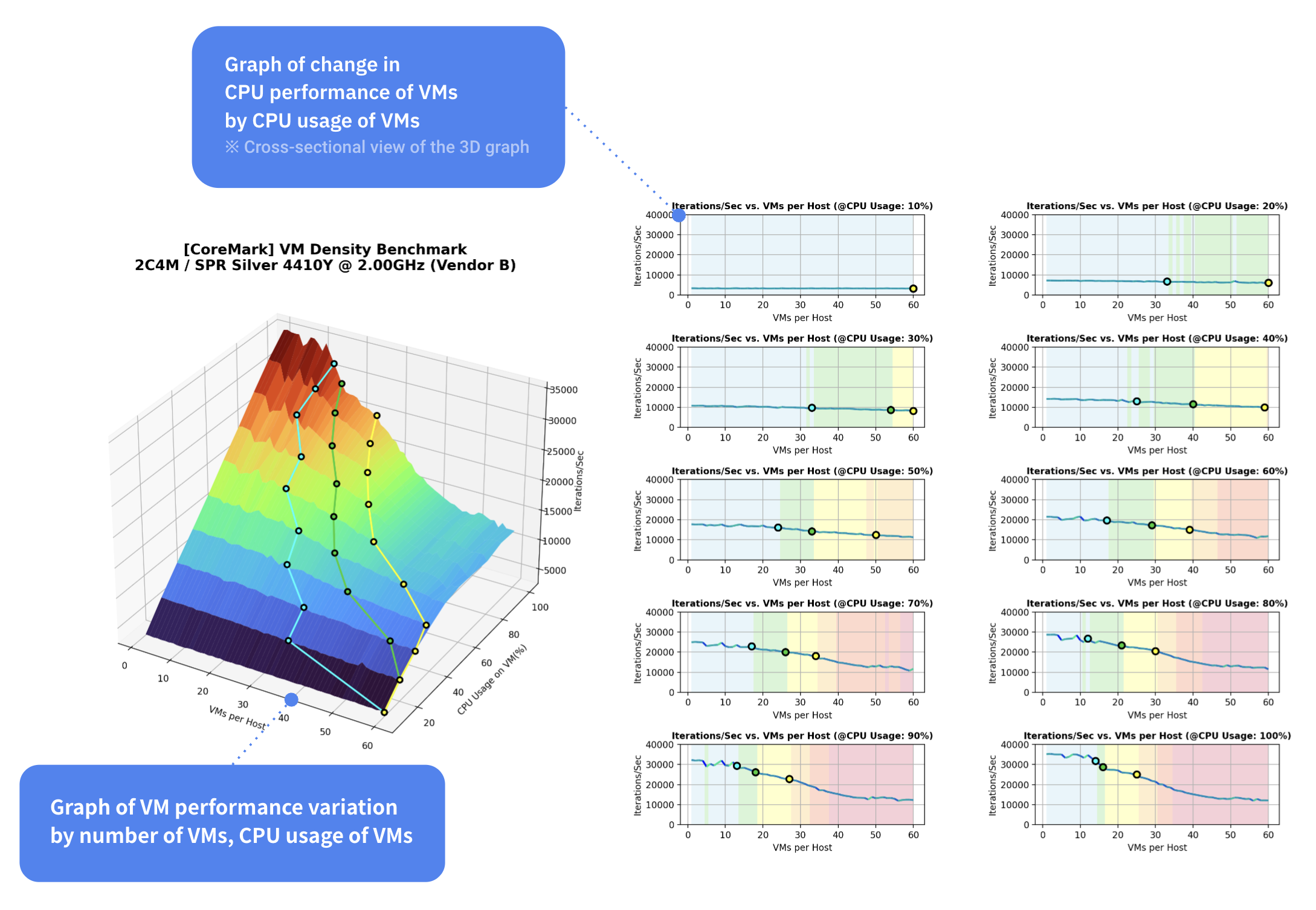
For each combination of PM specifications and VM flavor, the results consist of one 3D graph and ten 2D graphs, as shown in the figure above. As mentioned earlier, the tests were conducted by running the benchmark program on multiple VMs simultaneously for each condition, and CoreMark was used as the benchmark program.

Iterations/Sec is the average value of the benchmark results for each VM, indicating the CPU performance of the VM. It’s important to note that the benchmark result, Iterations/Sec, doesn’t mean much by itself. For example, just because a result at 10% CPU usage is lower than the result at 100% CPU usage does not mean that the VM is actually performing worse. Also, just because the highest result is when there is only one VM and the VM is at 100% CPU usage does not mean that the optimal VM density is 1. Because the benchmark program was run with a limit on the VM’s CPU usage, it is natural for the result at 10% CPU usage to be lower than the result at 100% CPU usage.

The reason for limiting a VM’s CPU usage is that, as mentioned earlier, in the actual operating environment, not all VMs will use 100% of their CPU all the time. The goal of the test was to determine the maximum number of VMs that can coexist in the actual operating environment without affecting each other’s performance, given that the VMs are using XX% CPU on average. To accomplish this, I used the results for a single VM (on the far left) as a baseline, i.e. the performance that a VM should have with no contentions, and saw how many more VMs could be added to the PM while maintaining that performance.

3D Graph (Graph of overall change in CPU performance of VMs)

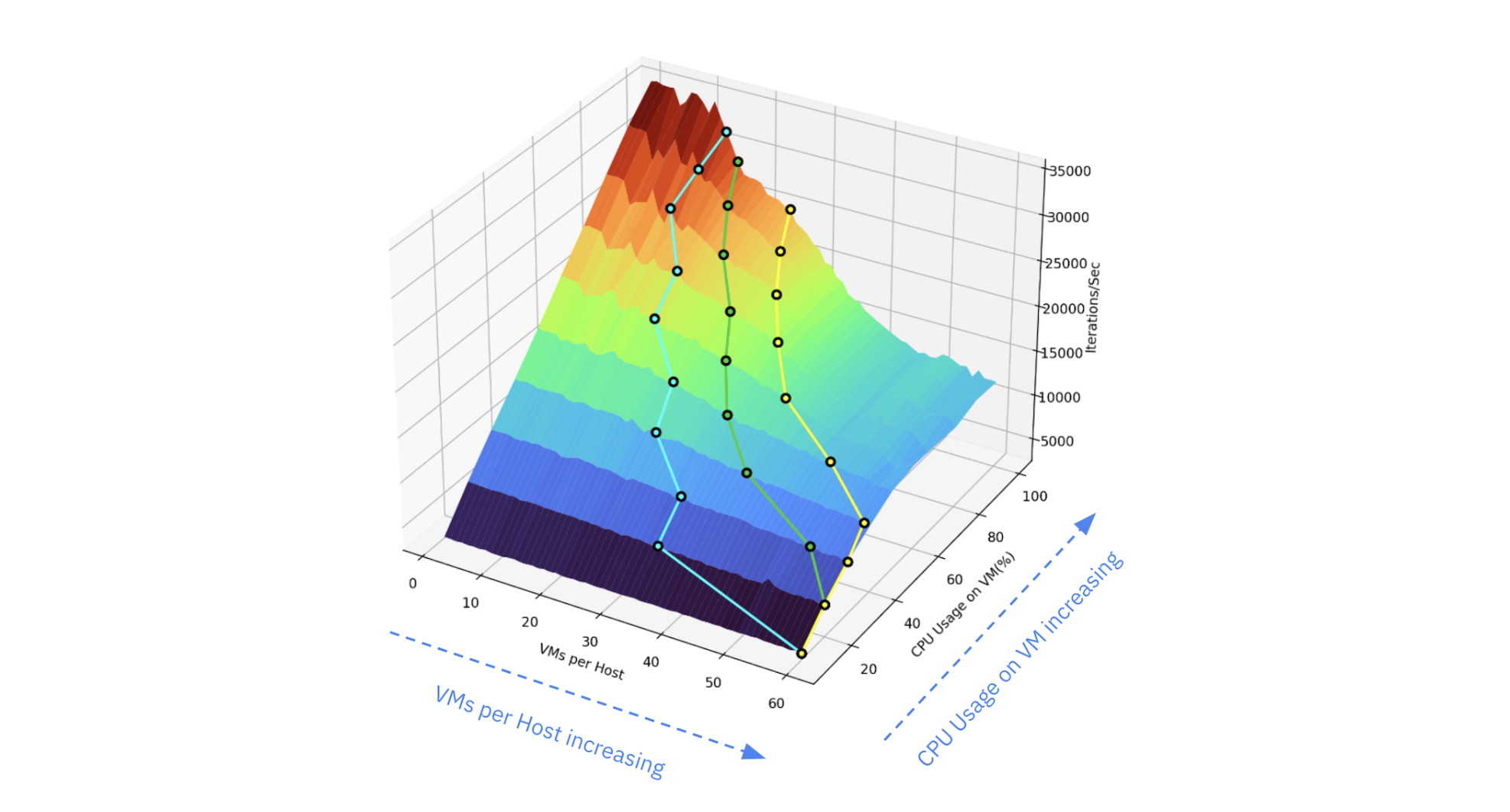
A 3D graph with the number of VMs on the x-axis, CPU usage of VMs on the y-axis, and benchmark results on the z-axis. It provides an overview of how a VM’s CPU performance varies with the number of VMs and the VM’s CPU usage.

2D Graph (Graph of change in CPU performance of VMs by CPU usage of VMs)

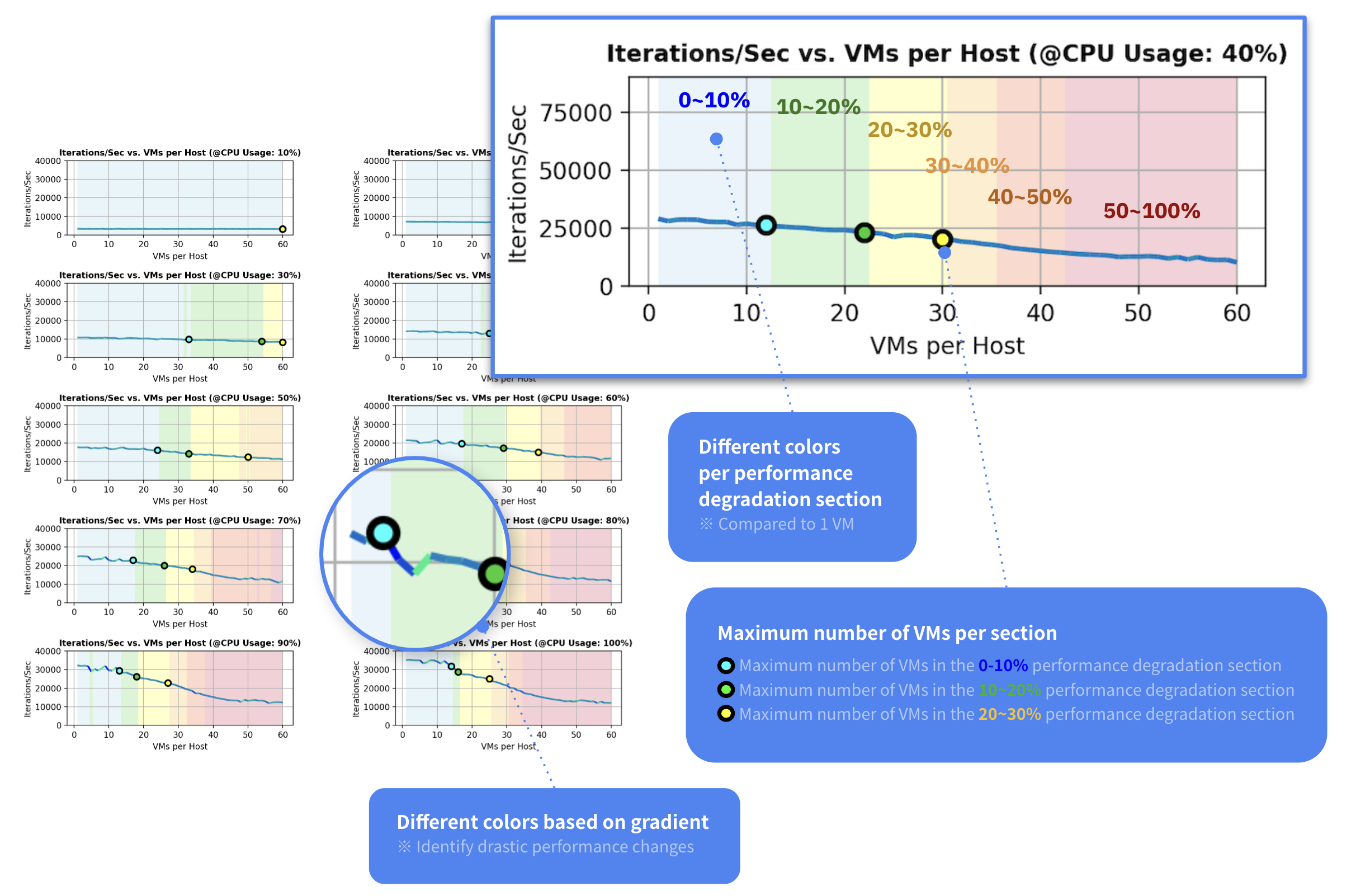
These 2D graphs are cross-sectional views of the 3D graph introduced earlier for each of the VM’s CPU usage (10%, 20%, 30%, … 100%).

What each of these graphs represents is the change in VM performance as the number of VMs increases for each percentage of CPU usage. In other words, these graphs enable understanding of ‘how many VMs start to see a decrease in performance when the average CPU usage of the VMs is at XX%’.

For easy identification of how much the CPU performance of the VM decreased, color sections are divided according to the performance degradation rate compared to the benchmark result when there was only one VM (on the far left). The performance degradation rate range for each section is as follows.

• 0 ~ 10%
• 10 ~ 20%
• 20 ~ 30%
• 30 ~ 40%
• 40 ~ 50%
• 50% ~

In addition, for the three sections, 0 - 10%, 10 - 20%, and 20 - 30%, there are additional markings on the rightmost numbers of VMs for each section. These markings represent the maximum number of VMs that can be accommodated in one PM, assuming that the CPU performance degradation of the VM can be tolerated up to 0 - 10%, 10 - 20%, and 20 - 30%.

Furthermore, the graph is colored differently based on the gradient of the graph to make it easier to see when a VM’s CPU performance is dropping rapidly (closer to darker blue means more drastic performance degradation).

2) Analysis of VM’s CPU Performance Variation

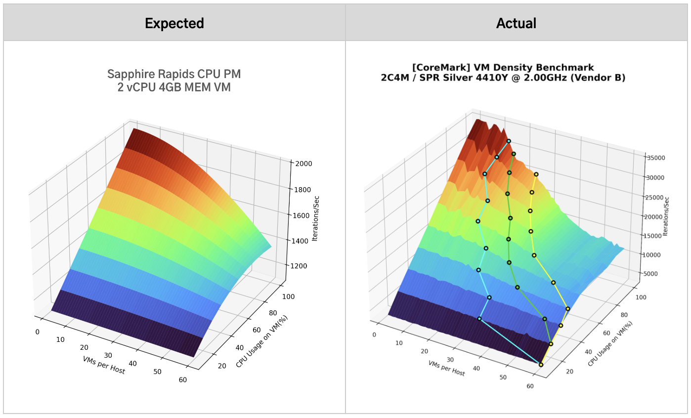
In the case of the 3D graph, results similar to the graph expected before conducting the test were obtained. The benchmark scores decreased as more VMs used more CPU resources, due to the increased contention for the limited CPU resources of the PM.

Especially, when the number of VMs is small enough to use as much of the CPU resources of the PM as desired, increasing the CPU usage limit directly leads to an improvement in benchmark scores. However, when the number of VMs is large, the benchmark scores do not increase even if the CPU usage limit is increased, due to resource contention with other VMs. This expectation was consistent with the results.

The results are also consistent with the expectation that when VMs are using less CPU, PM’s CPU resources are relatively free, so increasing the number of VMs would not cause a significant decrease in benchmark results.

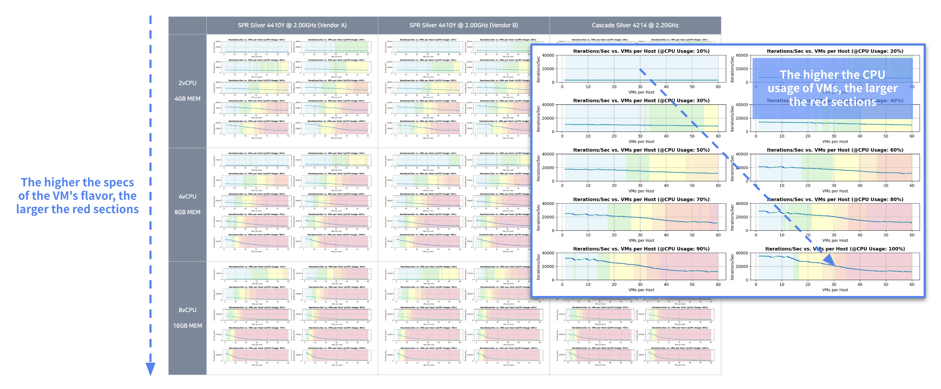
In the case of 2D graphs, the results were also overall as expected.

Looking at the overall results in terms of the flavor of the VM, the more high spec the flavor of the VM is (the higher the number of vCPUs in the VM), the less blue/green/yellow colors representing small performance decreases, and more red. This means that the higher the specs of the VM flavors, the greater the performance decrease, even for a small number of VMs.

Likewise, when looking at the results for each combination of PM and VM flavor in terms of CPU usage of the VMs, as the CPU usage of the VMs increases, the color of the small performance decrease sections (blue/green/yellow) decreases, while the red increases. This means that the higher the CPU usage of the VMs, the greater the performance decrease even for a small number of VMs.

In conclusion, it can be observed that the more low spec the flavor of the VM, and the lower the CPU usage of the VM, the better performance is maintained as the number of VMs increases.

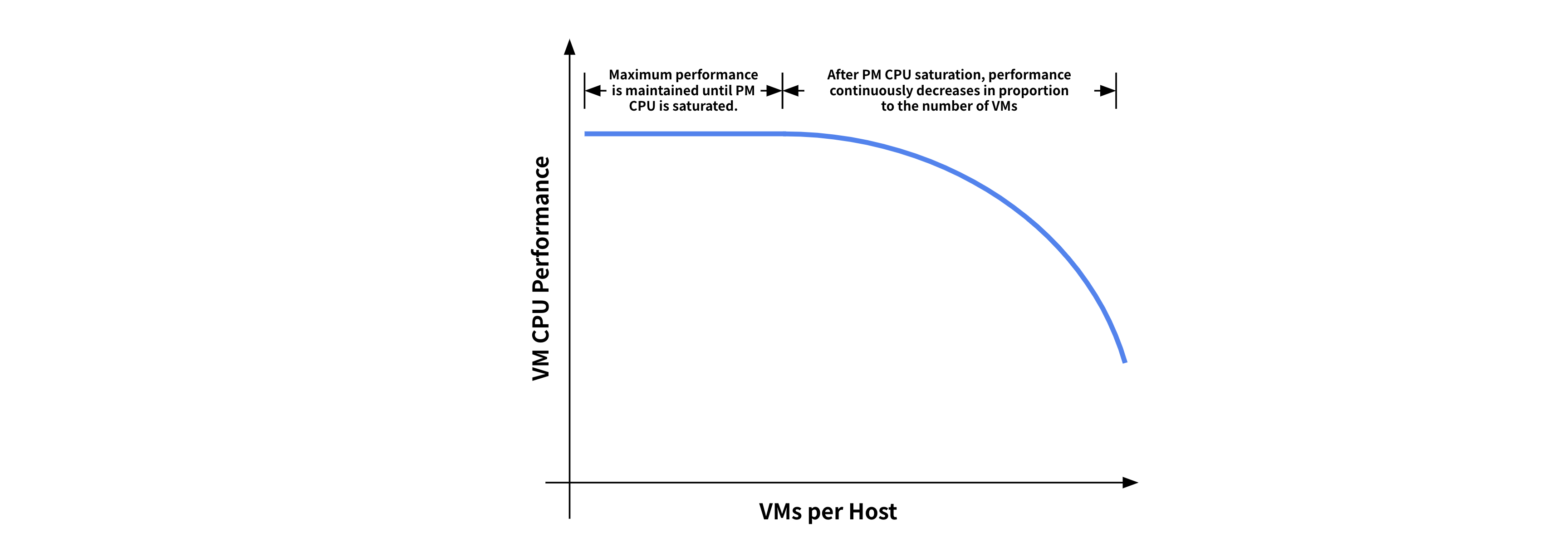
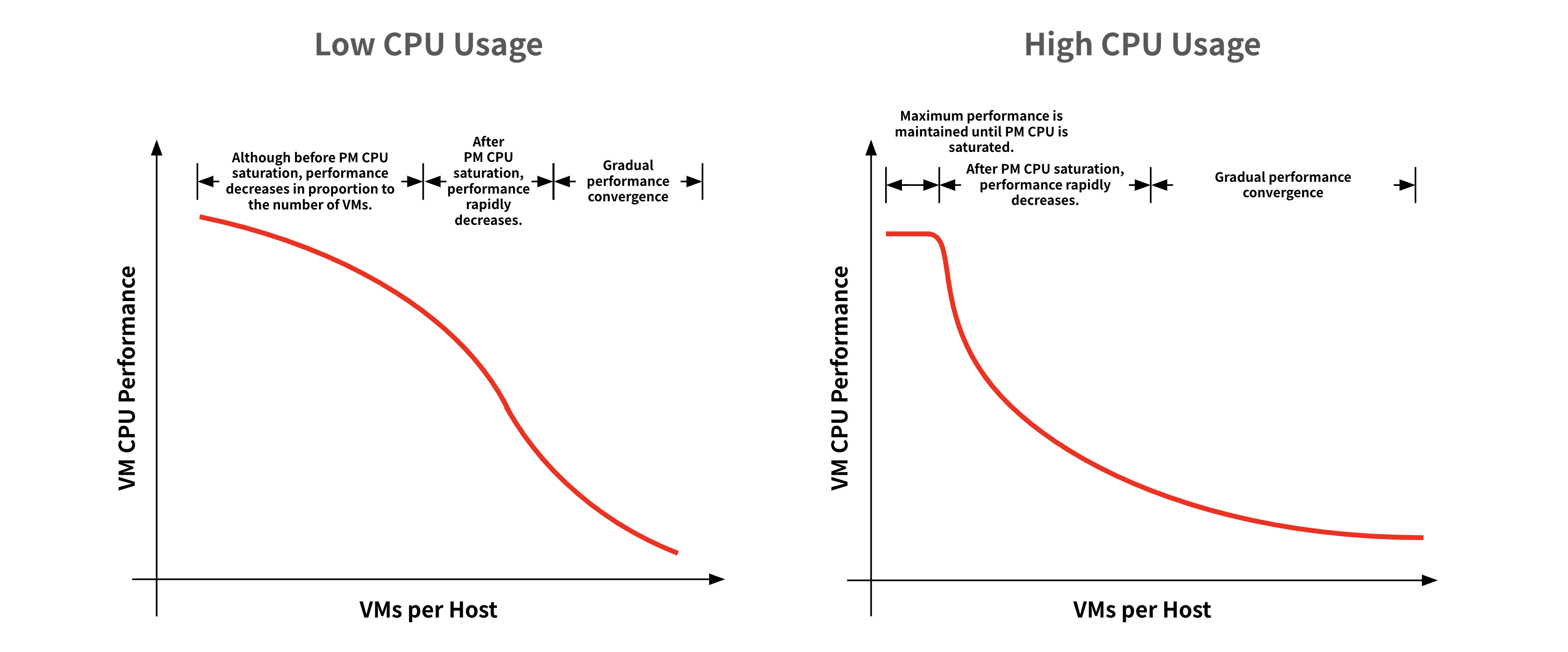
Overall, the results were not much different from expectations. However, some of the details were not as expected. Let’s look at the graph by splitting it into low and high CPU usage for the VMs.

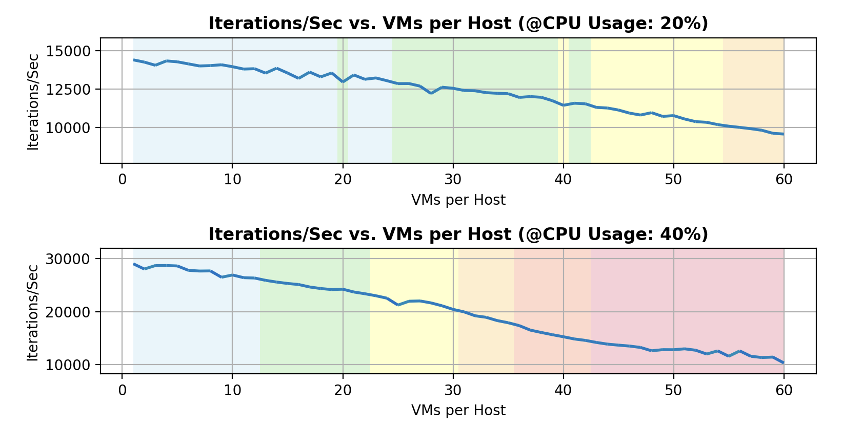
First, for low VM CPU usage, contrary to expectations that lower VM CPU usage would result in better performance maintenance, there was a significant performance degradation from a small number of VMs.

Of course, the performance degradation is lower than when the VM’s CPU usage is high, but it does mean that even when the PM’s CPU resources are free, there is a performance degradation due to the effects of other VMs.

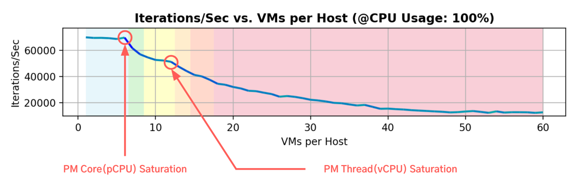
For high VM CPU usage, the point at which CPU performance started to degrade was earlier than expected.

With Hyper-Threading enabled, the performance was expected to be maintained as the number of VMs increased until PM’s threads (vCPUs) were saturated, but after PM’s cores (pCPUs) were saturated, there was a significant performance degradation.

And overall, regardless of the CPU usage of the VMs, the performance decreased rapidly once it started, and then slowed down after a certain point, contrary to the expectation that CPU performance would decrease proportionally as the number of VMs increased. In other words, the performance variation was closer to 1/N (N = number of VMs) than expected.

4. Factors that affect CPU performance degradation in VMs

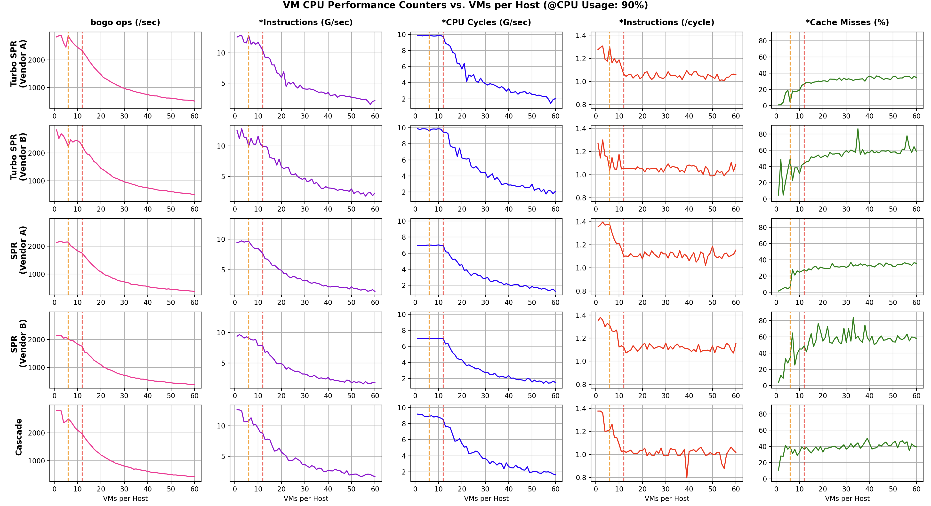
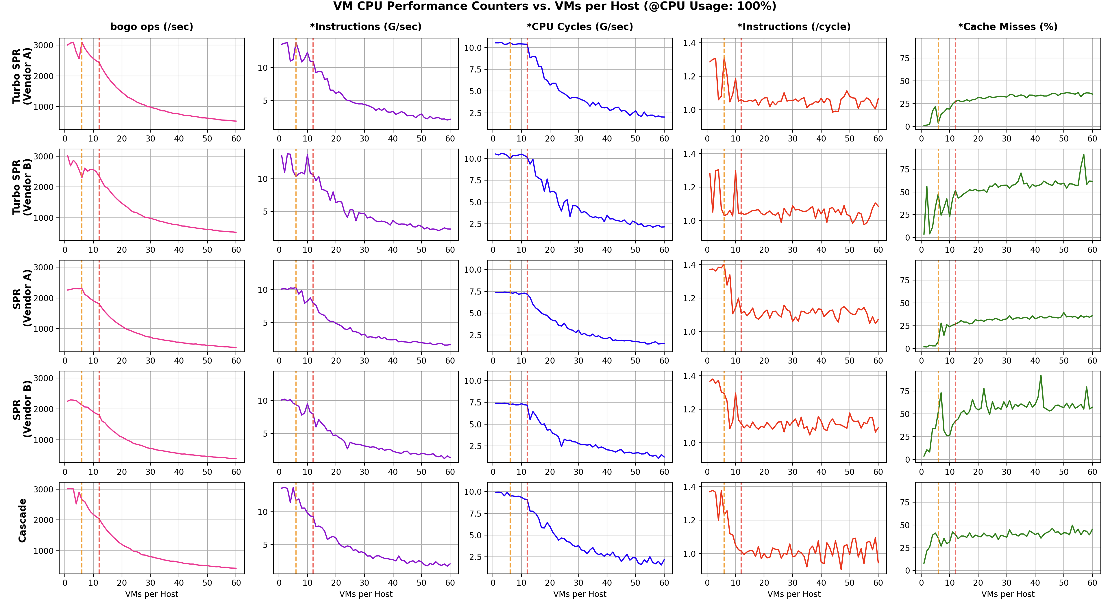
1) Data Overview

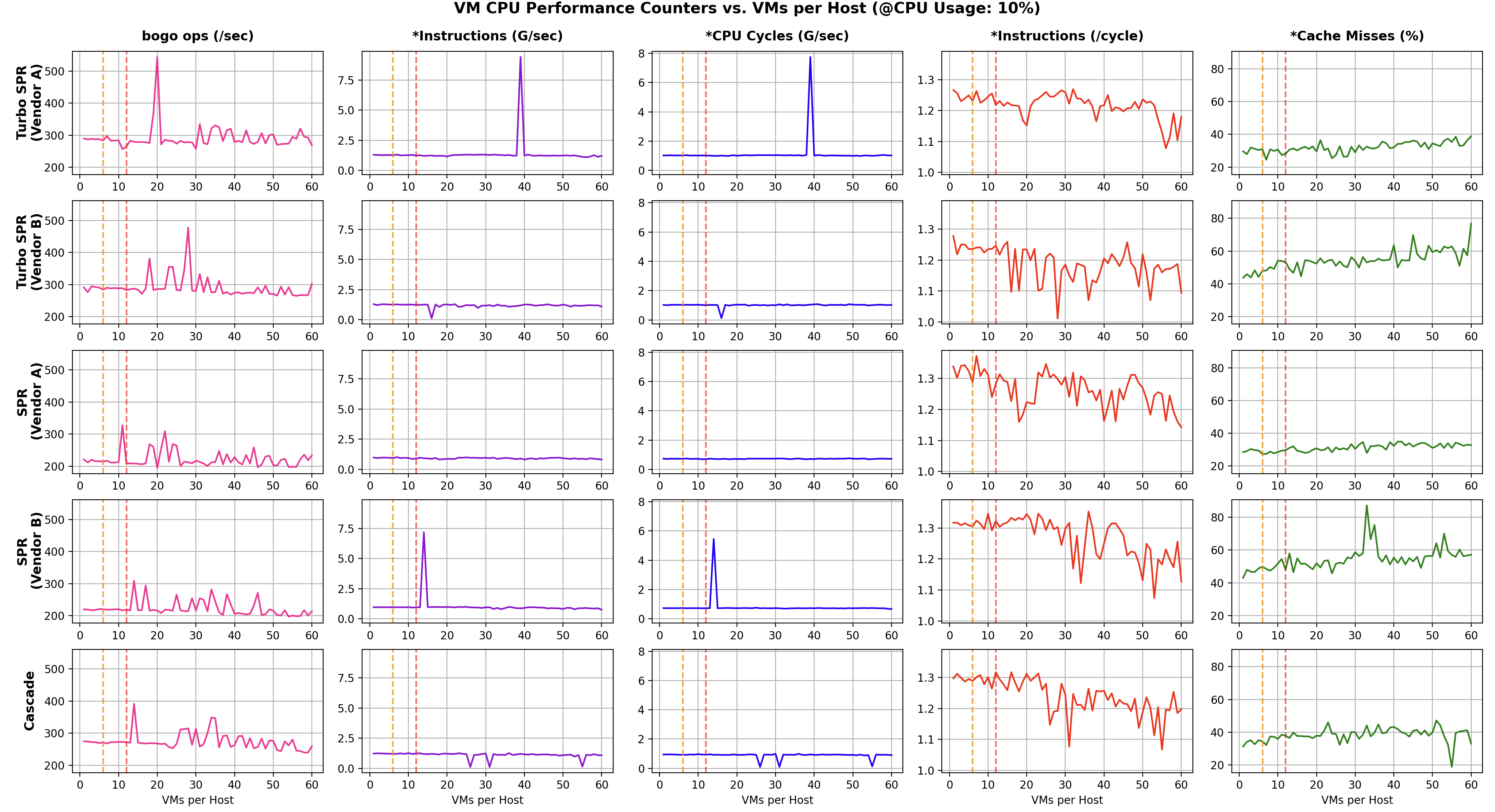
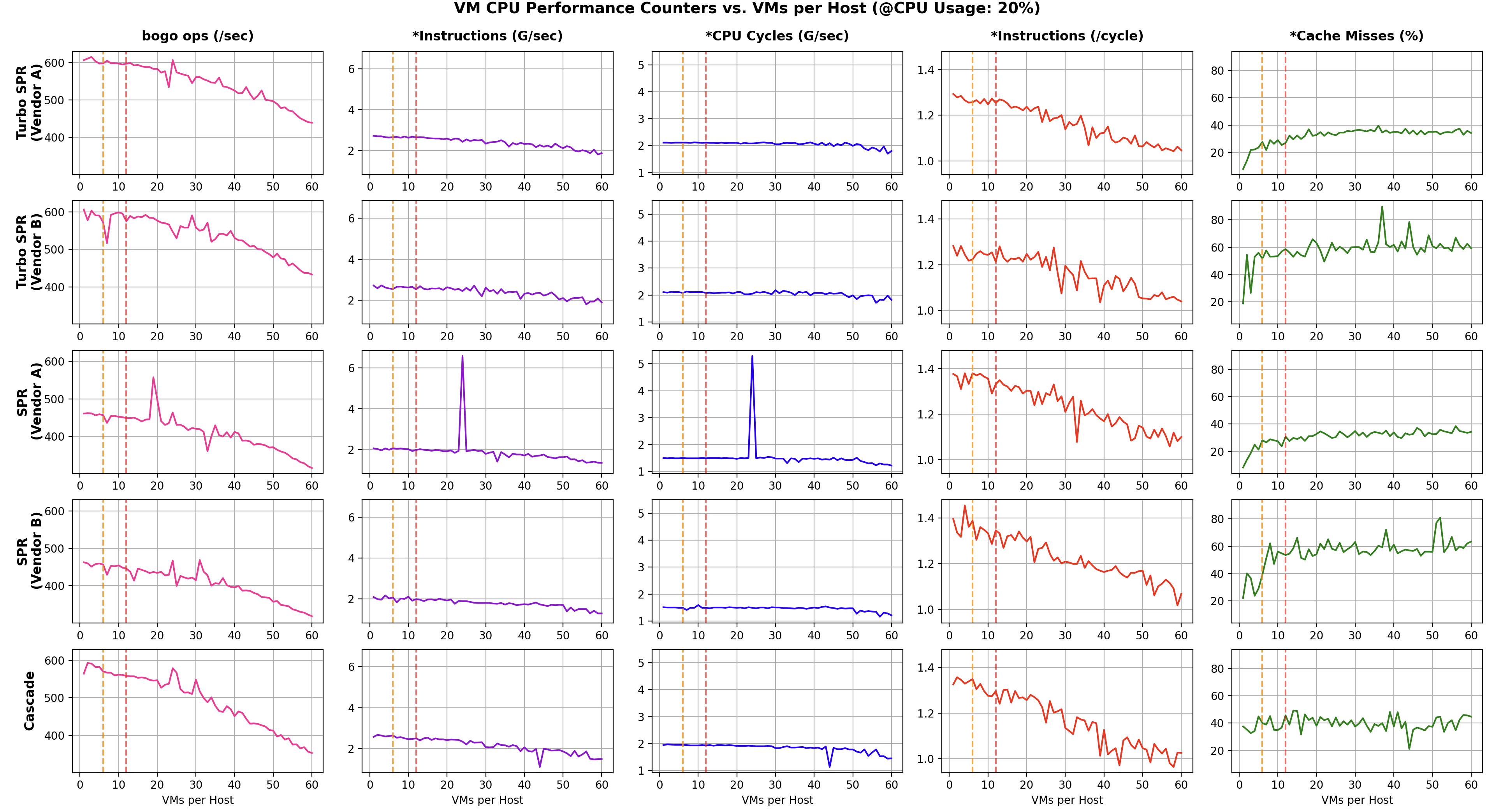
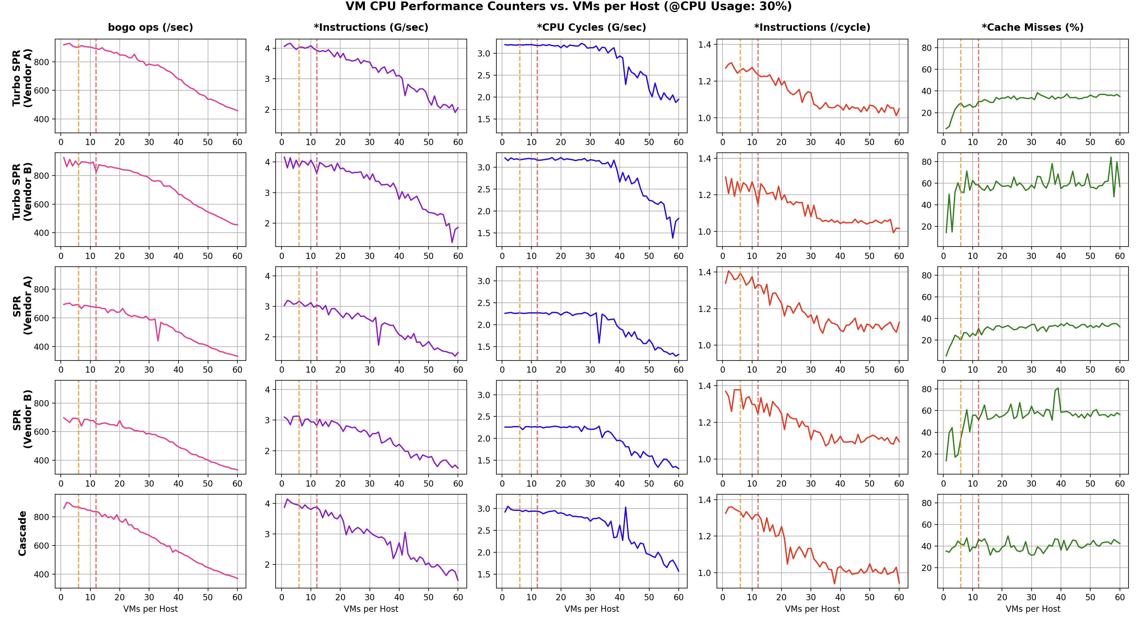
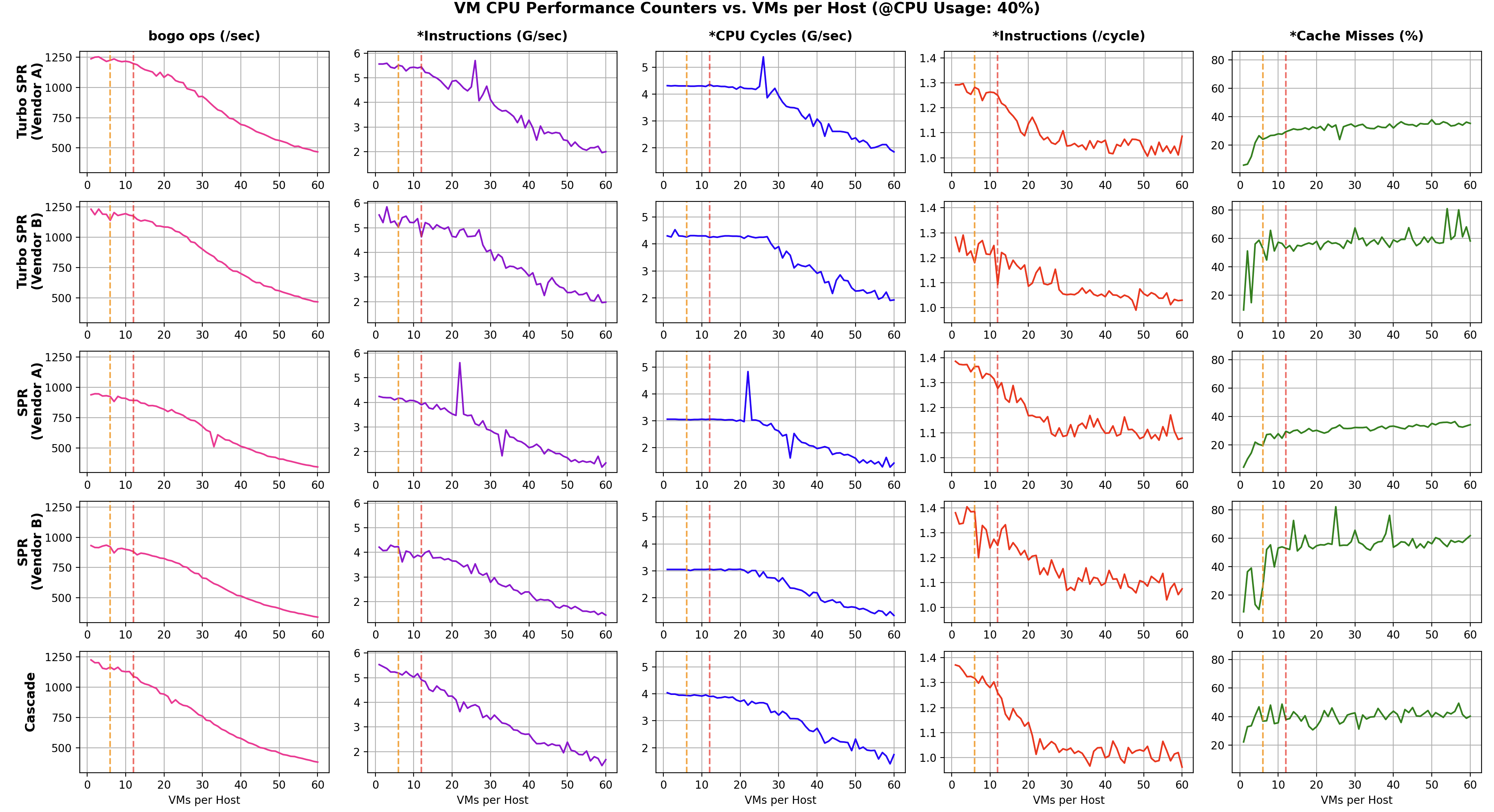
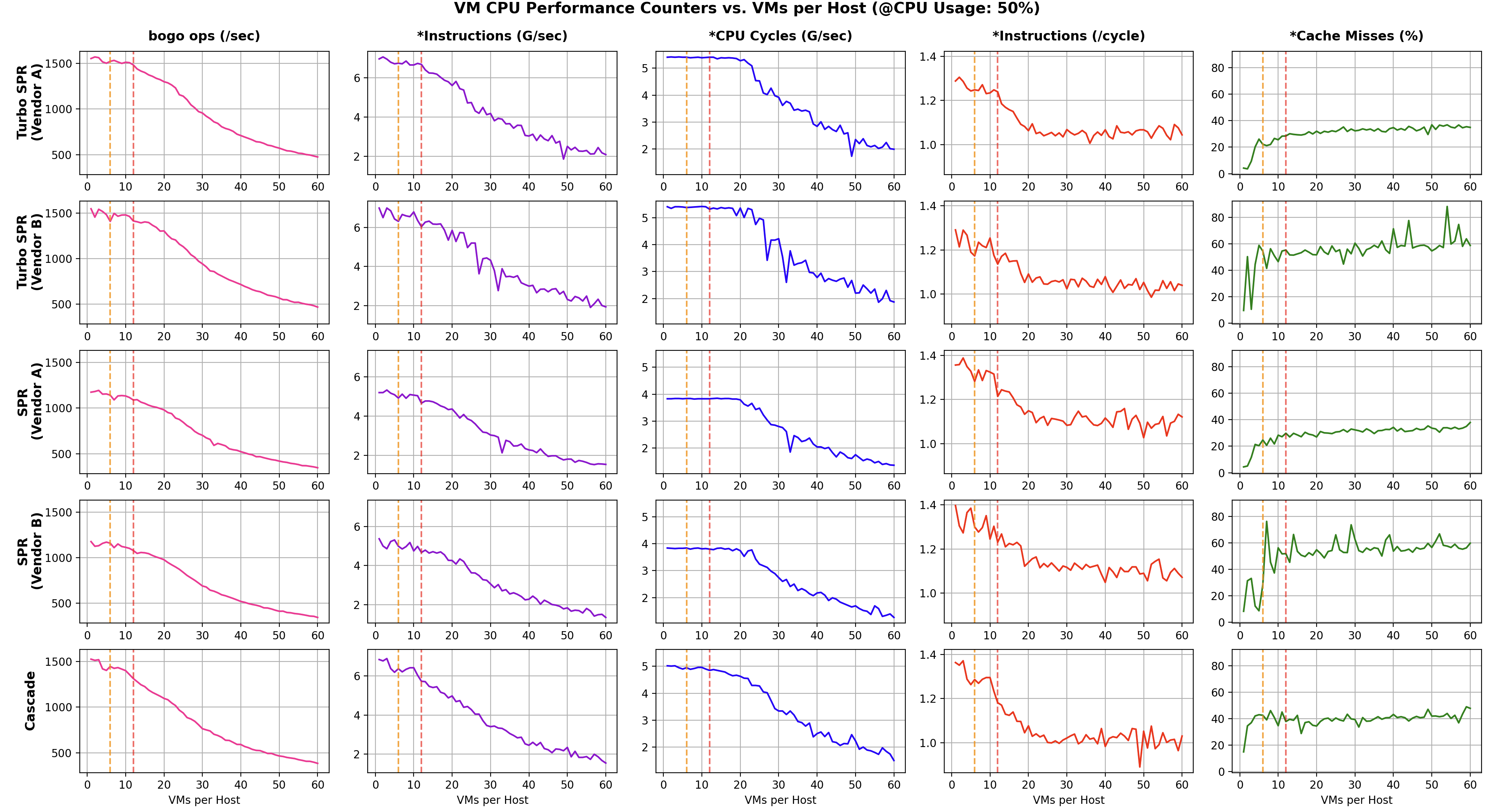
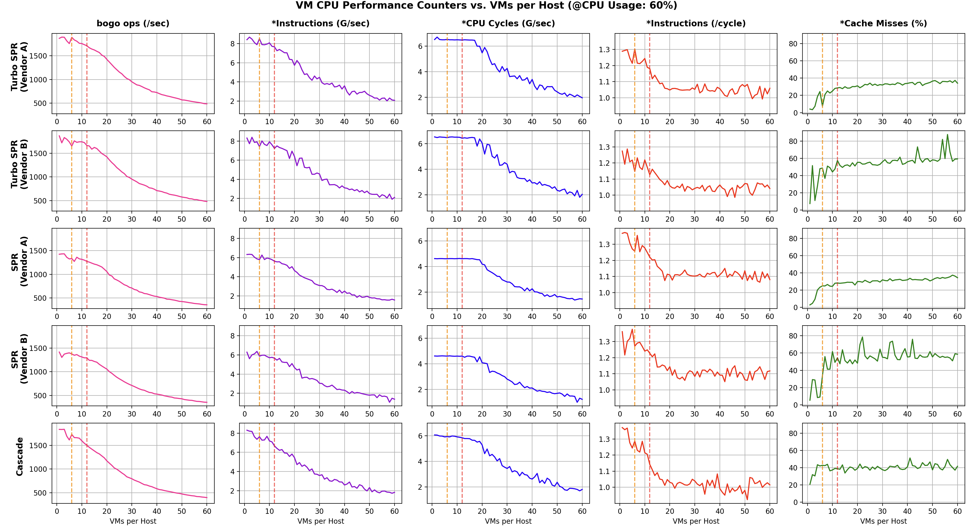
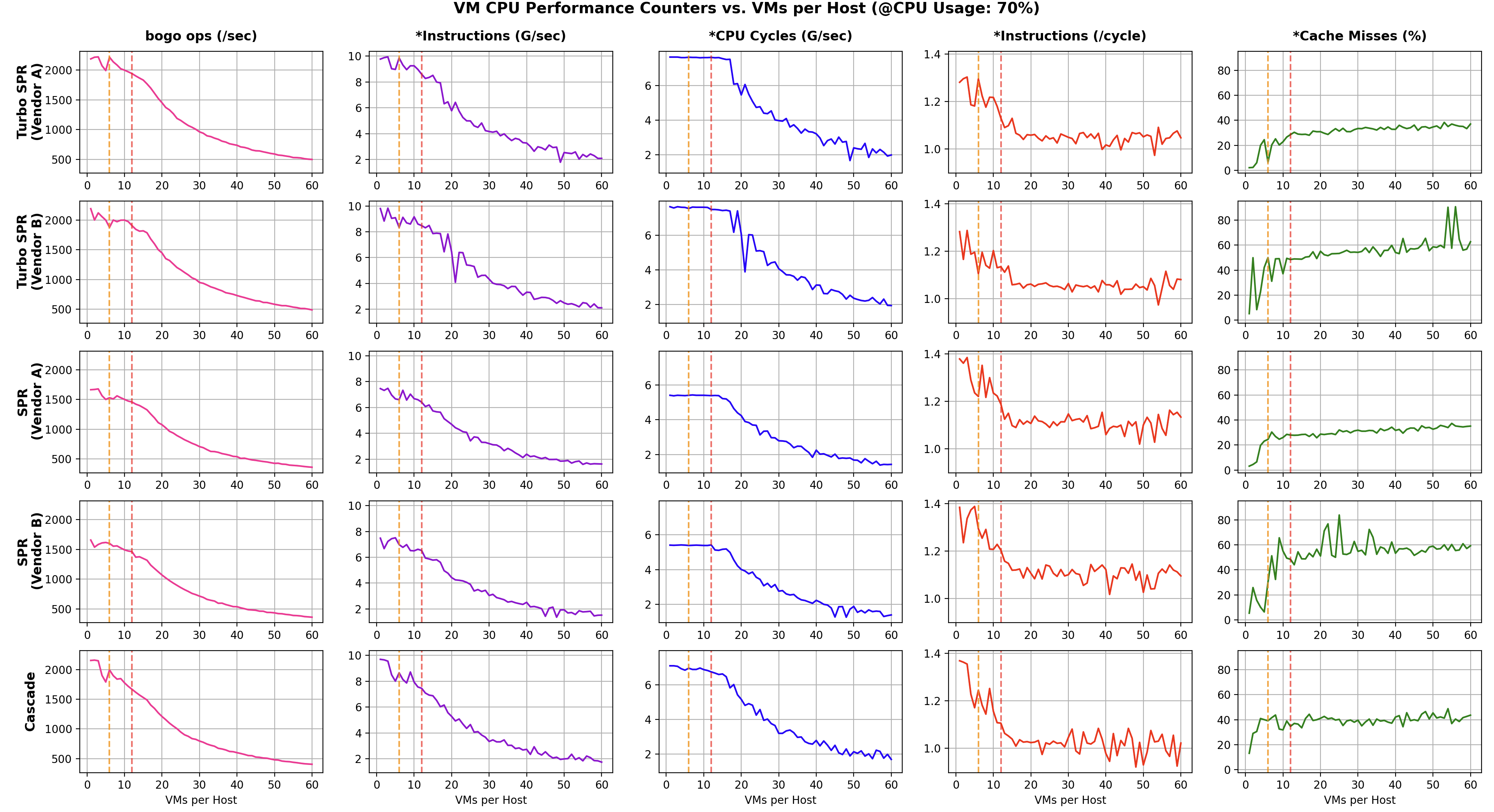
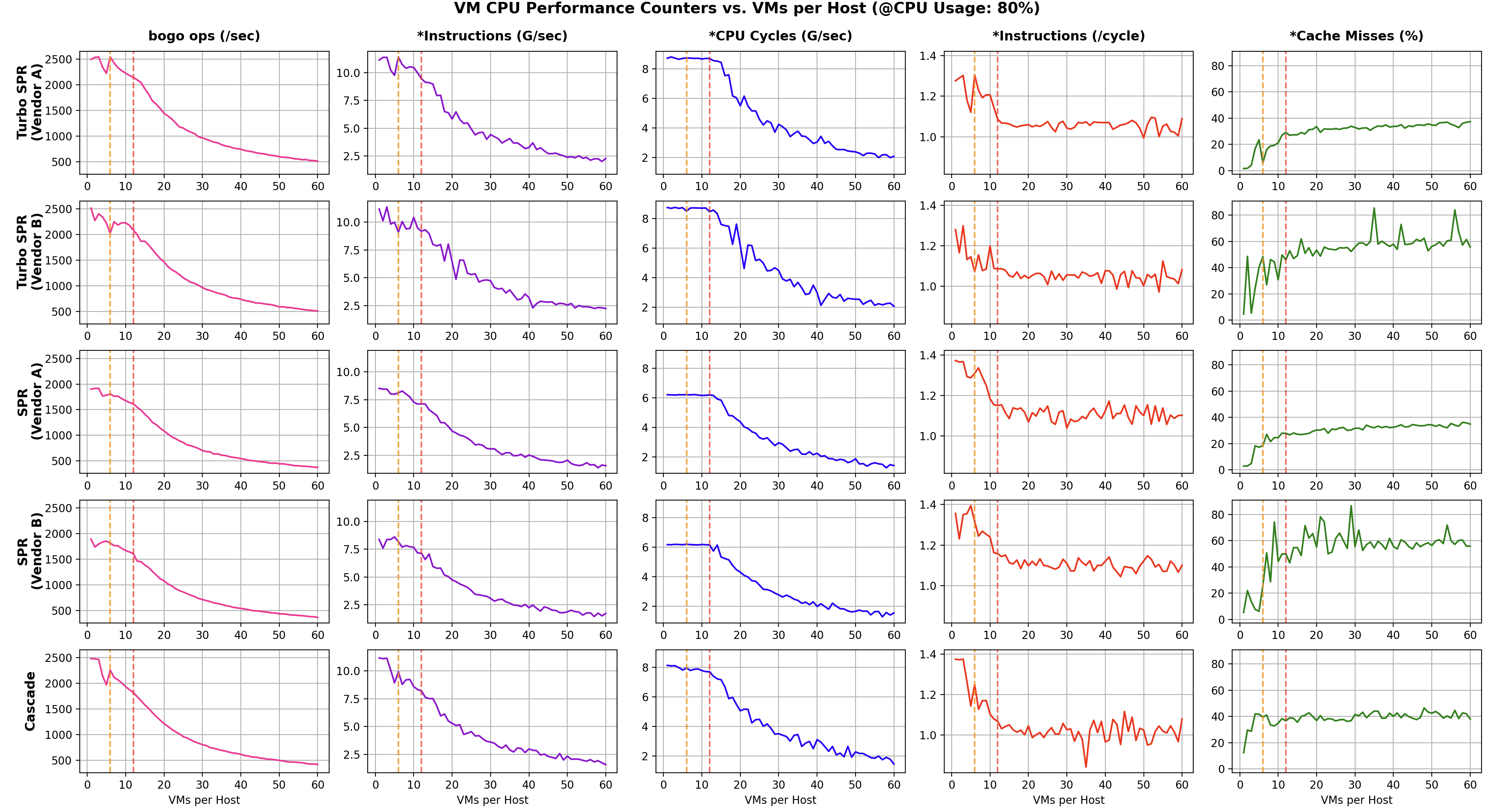
This is a more detailed analysis of the previous section ‘3. Changes in CPU performance of VMs as the number of VMs increases’. It shows the change in the CPU performance counter of a VM as the number of VMs increases when the VM’s CPU usage is 10%, 20%, 30%, … 100% for each.

Additional tests were conducted to understand what happens internally as the number of VMs increases and what ultimately leads to the decrease in CPU performance of the VMs. The test method is the same as before, but with the difference that it was only conducted on a 4 vCPU / 8GB MEM flavor VM and used a benchmark program called stress-ng. To get the CPU performance counter values for the VM, the --perf option of stress-ng was used.

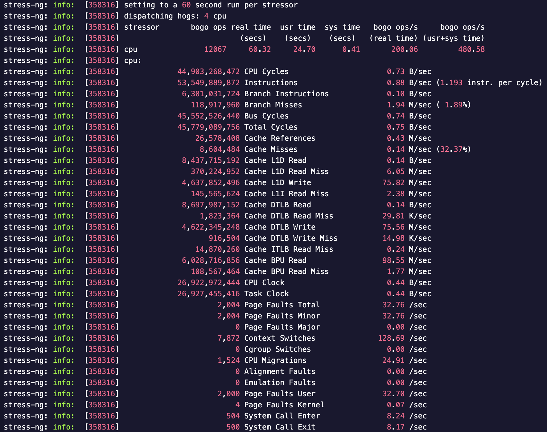
Using the --perf option of stress-ng, CPU performance counter statistics are output along with the benchmark results, as shown above.

Based on the test results of varying the CPU usage of the VMs for each PM, the final graph is shown below.

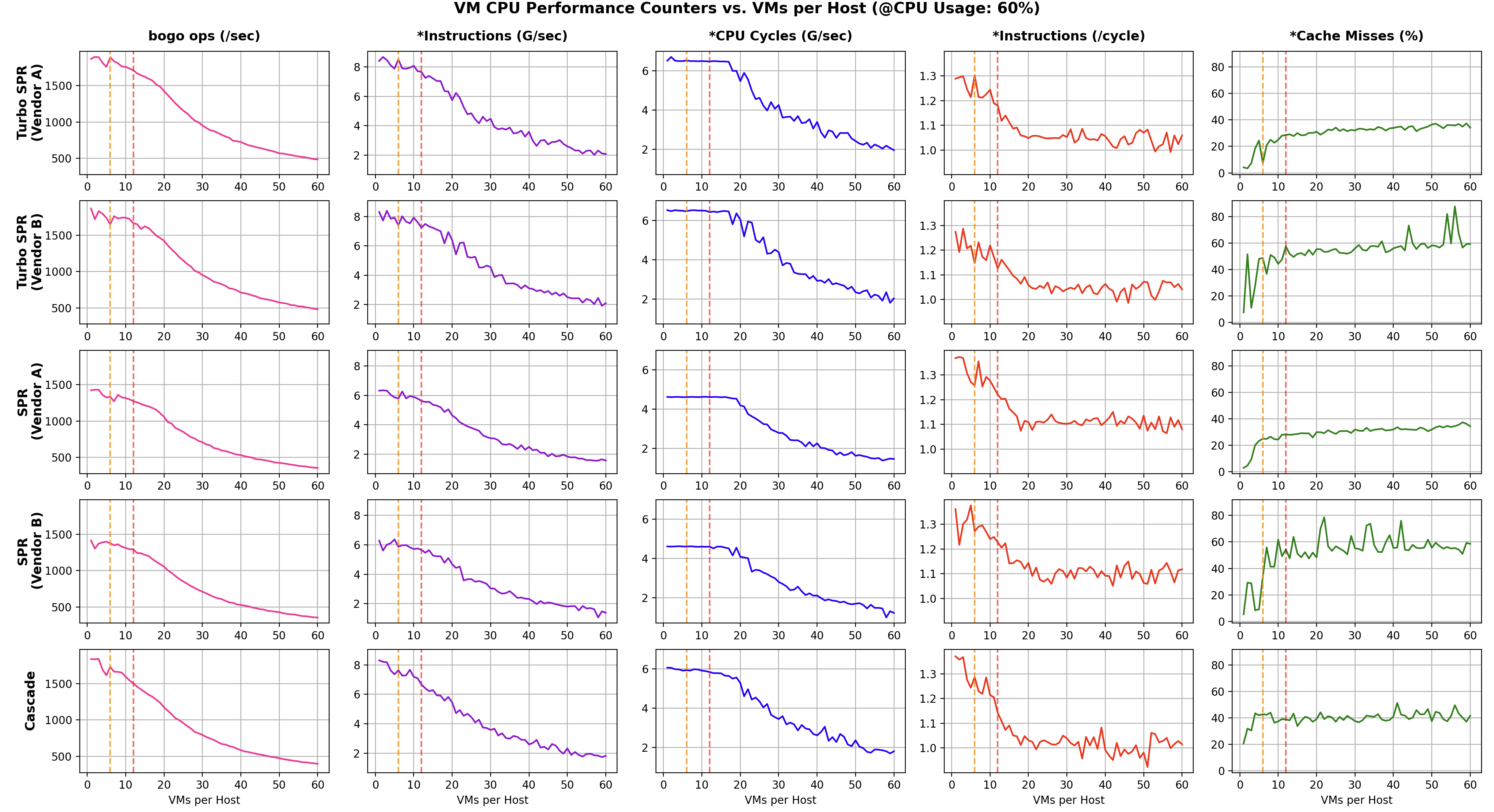
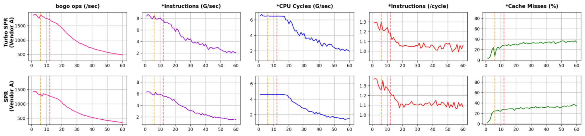
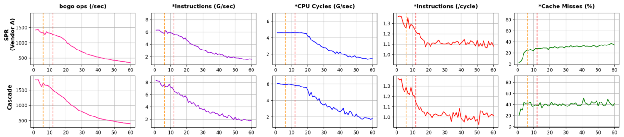
Each row corresponds to a specific PM, and each column represents the benchmark results and the value of the VM’s CPU performance counter.

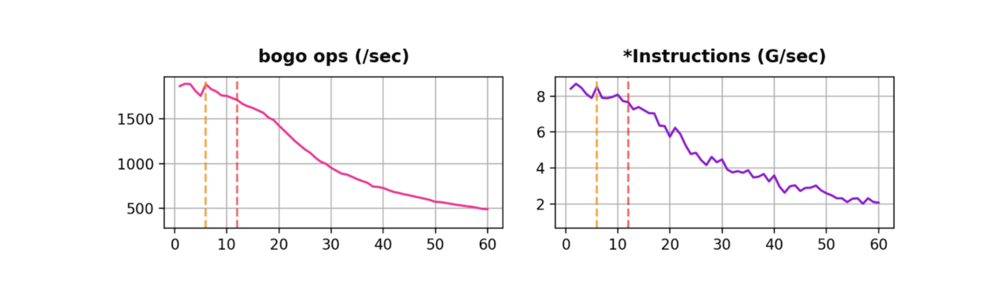
bogo ops(/sec) is the average of the results of running the stress-ng benchmark (cpu-method=all) on N VMs simultaneously.

The other entries starting with * are the sampled VM CPU performance counter values, which were extracted from only one VM, even though the actual benchmark was run on N VMs simultaneously. To collect the CPU performance counter values of a VM, it is necessary to enable the Virtual CPU Performance Counters feature, but due to the difficulty of setting it for all VMs, it is only applied to one VM per PM.

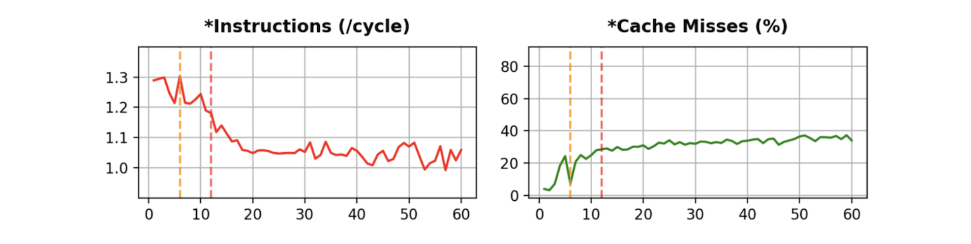
The orange dashed line shows the number of VMs where the number of cores (pCPUs) in the PM equals the sum of the number of vCPUs in the VMs (24 ÷ 4 = 6), and the red dashed line shows the number of VMs where the number of threads (vCPUs) in the PM equals the sum of the number of vCPUs in the VMs (48 ÷ 4 = 12).

2) Graph Analysis

bogo ops(/sec) ≒ Instructions(G/sec)

• The bogo ops(/sec) graph and the Instructions(G/sec) graph have similar shapes.

• The results of the benchmark, which is the CPU performance of the VM, can be seen to follow the Instructions(G/sec) value.

• The reason the Instructions(G/sec) graph appears unstable compared to the bogo ops(/sec) graph is because it is sampled from only one VM, unlike bogo ops(/sec), which is averaged over N VMs.

Instructions(G/sec) = CPU Cycles(G/sec) × Instructions(/cycle)

• Instructions(G/sec) can be represented as the product of CPU Cycles(G/sec) and Instructions(/cycle).
• In other words, even if the CPU Cycles(G/sec) remains the same, but Instructions(/cycle) decreases, or conversely, if Instructions(/cycle) remains the same, but CPU Cycles(G/sec) decreases, Instructions(G/sec) will decrease.

Relationship between CPU Cycles(/sec) and Instructions(/cycle)

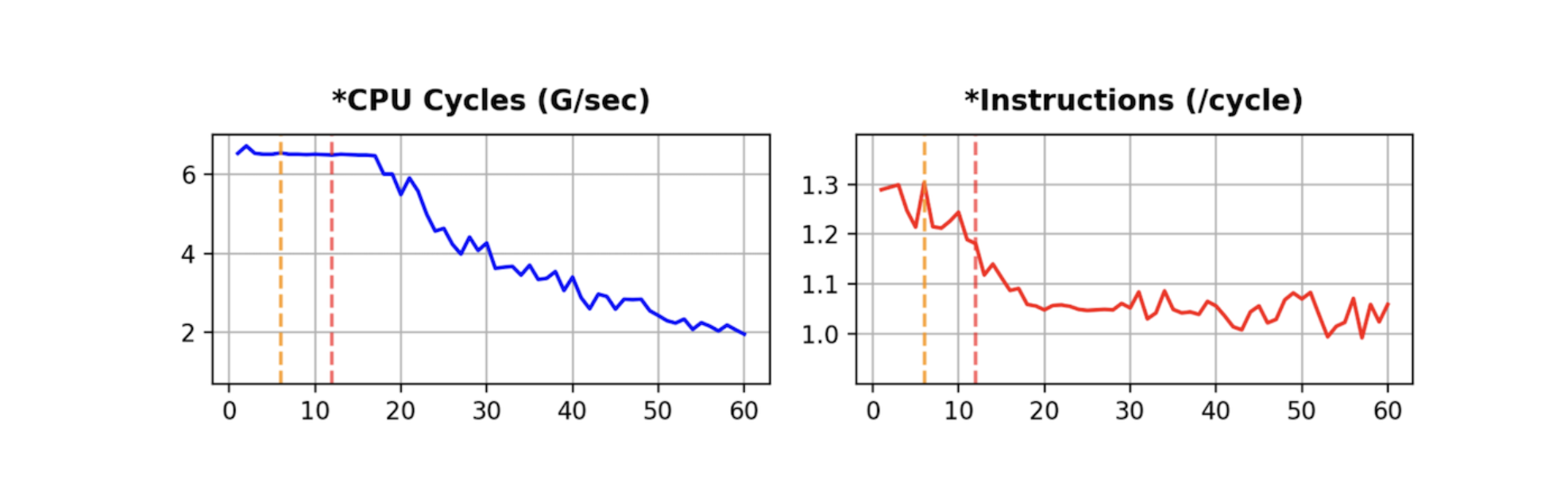
• Instructions(/cycle) and CPU Cycles(/sec) never decrease at the same time.
• When Instructions(/cycle) starts to decrease, CPU Cycles(/sec) starts to decrease.

CPU Cycles(G/sec)

• CPU Cycles(G/sec) is the sum of the number of cycles per second for each vCPU in the VM (in this case, there are 4 vCPUs, so the number of cycles per vCPU can be calculated by dividing by 4).

• CPU Cycles(G/sec) tends not to decrease, at least until the sum of the number of vCPUs in the VM equals the number of threads(vCPUs) in the PM (before the red dotted line).

• The lower the CPU usage of the VM, the longer the CPU Cycles(G/sec) tends to be maintained even after the sum of the VM’s vCPUs exceeds the PM’s threads(vCPUs), because the lower the CPU usage of the VM, the more CPU resources are freed up in the PM.

• In other words, when CPU Cycles(G/sec) starts to decrease, it means that the PM’s CPU resources are saturated, and from that point on, CPU Cycles(G/sec) is the cause of the decrease in Instructions(G/sec) (≒ bogo ops(/sec)).

Instructions(/cycle)

• Instructions(/cycle) is the sum of the number of instructions executed in one CPU cycle for each vCPU in the VM.

• Instructions(/cycle) initially decreases steadily as the number of VMs increases, and then converges after a point.

• That point is the same as when CPU Cycles(G/sec) starts to decrease, which means that Instructions(/cycle) will decrease until the PM’s CPU resources are saturated.

• In fact, the lower the CPU usage of a VM, the further Instructions(/cycle) tends to decrease after the sum of the VM’s vCPU count exceeds the PM’s Thread (vCPU) count, i.e. after it crosses the red dotted line.

• Since CPU Cycles(G/sec) does not decrease until the PM’s CPU resources are saturated, the decrease in Instructions(G/sec) (≒ bogo ops(/sec)) that occurs before the PM’s CPU resources are saturated can be attributed to Instructions(/cycle).

Cache Misses(%)

• Since this is a virtual CPU performance counter value for the VM, it’s hard to explain how it relates to the actual PM’s CPU cache, but it indicates the overall cache miss rate (%) for the VM (Cache Misses / Cache References).

• Cache Misses(%), regardless of the CPU usage of the VMs, initially increases significantly with the number of VMs and then stops increasing or increases very slowly after the sum of the number of vCPUs in the VMs exceeds the number of Threads (vCPUs) in the PM, i.e. after the red dotted line.

Relationship between Instructions(/cycle) and Cache Misses(%)

• Instructions(/cycle) tends to be inversely correlated to Cache Misses(%).

• As Cache Misses(%) increases, Instructions(/cycle) decreases, and conversely, as Cache Misses(%) decreases, Instructions(/cycle) increases.

• The graph shapes don’t match perfectly because there are factors other than Cache Misses(%) that affect Instructions(/cycle).

• However, if there is a noticeable change in Cache Misses(%), there is usually a corresponding change in Instructions(/cycle), indicating that Cache Misses(%) plays an important role in Instructions(/cycle).

Branch Misses(%)

• Branch Misses(%) was also checked, but it remained constant around 1.8% regardless of CPU specs, VM CPU usage, and number of VMs.

• Given the small change with increasing number of VMs and almost no difference between PMs, this value was deemed insignificant for this test and excluded from the results graph.

3) Causes of CPU performance degradation in VMs as the number of VMs increases

Decrease in Instructions(/cycle)

• This is where CPU Cycles(/sec) remains constant and Instructions(/cycle) decreases.

• The lower the CPU usage of the VM, the later the point at which Instructions(/cycle) stops decreasing, or equivalently, the later the point at which CPU Cycles(/sec) starts decreasing.

• In this interval, as the number of VMs increases, the CPU performance of the VMs decreases due to a decrease in Instructions(/cycle).

• One of the causes of the decrease in Instructions(/cycle) is an increase in Cache Misses(%).

• Cache Misses(%) increases significantly with the number of VMs initially, regardless of the CPU usage of the VMs, and then hardly increases at all after the total number of vCPUs in the VMs exceeds the number of Threads (vCPUs) in the PM.

Decrease in CPU Cycles(/sec)

• This is where Instructions(/cycle) stops decreasing and CPU Cycles(/sec) starts decreasing.

• The higher the CPU usage of the VM, the earlier the point at which Instructions(/cycle) stops decreasing, or equivalently, the point at which CPU Cycles(/sec) starts decreasing.

• In this interval, the CPU performance of the VMs decreases due to a decrease in CPU Cycles(/sec) as the number of VMs increases.

• For Cache Misses(%), it is unlikely that Cache Misses(%) is responsible for the decrease in Instructions(/cycle) because it hardly increases after the sum of the VM’s vCPU count exceeds the PM’s Thread (vCPU) count.

4) Performance differences with and without Turbo Boost mode enabled

• When Turbo Boost mode is enabled (a feature supported by Intel CPUs), CPU Cycles(/sec) tends to increase by about 35% and Instructions(/cycle) tends to decrease by about 8% compared to not enabling it.

• Instructions(/cycle) decreases slightly, but CPU Cycles(/sec) increases dramatically, which ultimately improves the performance of the VM’s CPU.

5) Differences in performance degradation due to CPU specs differences in PMs

• For CPU Cycles(/sec), Cascade Lake starts with a higher value compared to Sapphire Rapids, but after the number of VMs increases sufficiently, Cascade Lake and Sapphire Rapids have similar values.

• For Instructions(/cycle), Cascade Lake and Sapphire Rapids start with similar values, but after the number of VMs increases sufficiently, Sapphire Rapids has a value that is 10% higher than Cascade Lake.

• As a result, Cascade Lake shows a large performance decrease compared to Sapphire Rapids, which means that the optimal VM density results for Cascade Lake CPU PM in this test could be negatively impacted.

• However, it is not appropriate to compare two PMs with different CPU specifications in absolute numbers, as the benchmark results for each PM’s CPU specification can vary depending on the characteristics of the benchmark program.

6) Difference in Cache Misses(%) between Vendors

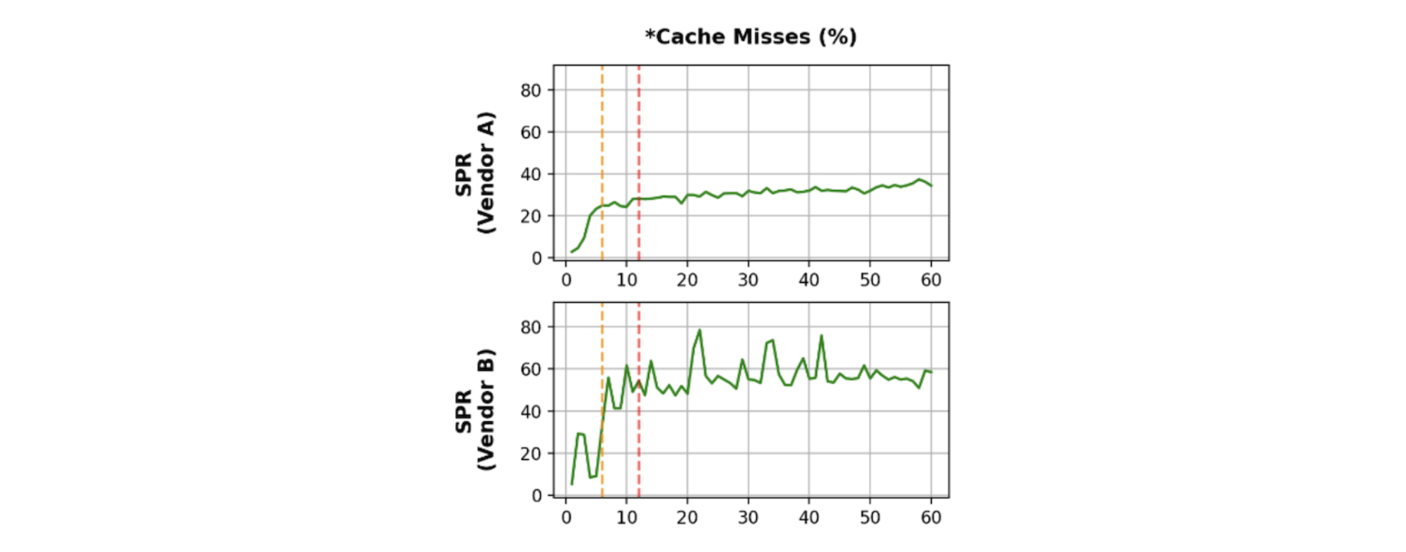
• Stable Cache Misses(%) trend on Vendor A equipment compared to Vendor B equipment.

• On Vendor B equipment, we see a large variation in Cache Misses(%), increasing by up to 60%.

• On the other hand, we see a smaller change in Cache Misses(%) on Vendor A equipment, with an increase of up to 40%.

• This means that even PMs with the same CPU model can have performance differences due to differences in overall equipment configuration across vendors.

5. Optimal VM Density

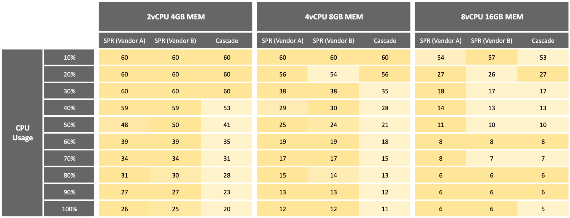
1) Data Overview

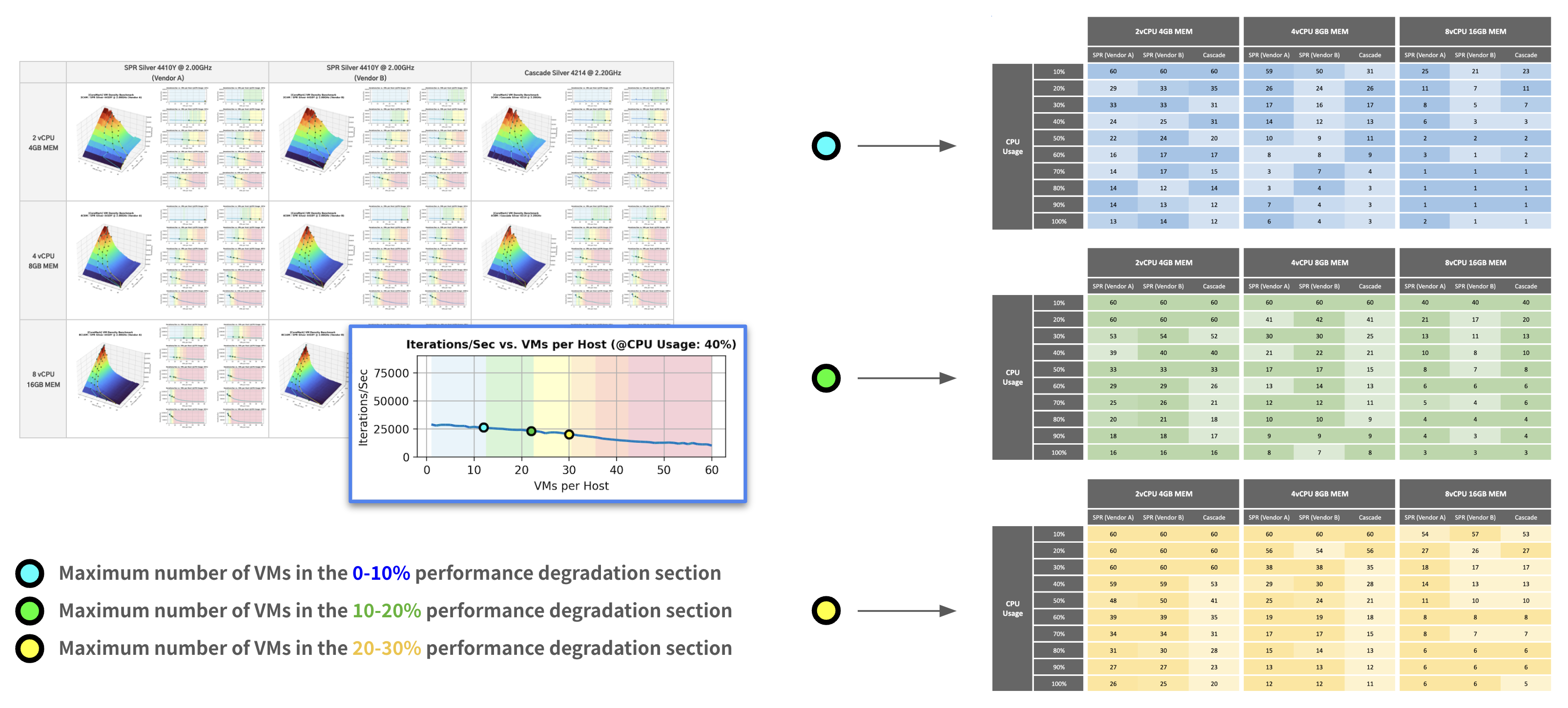
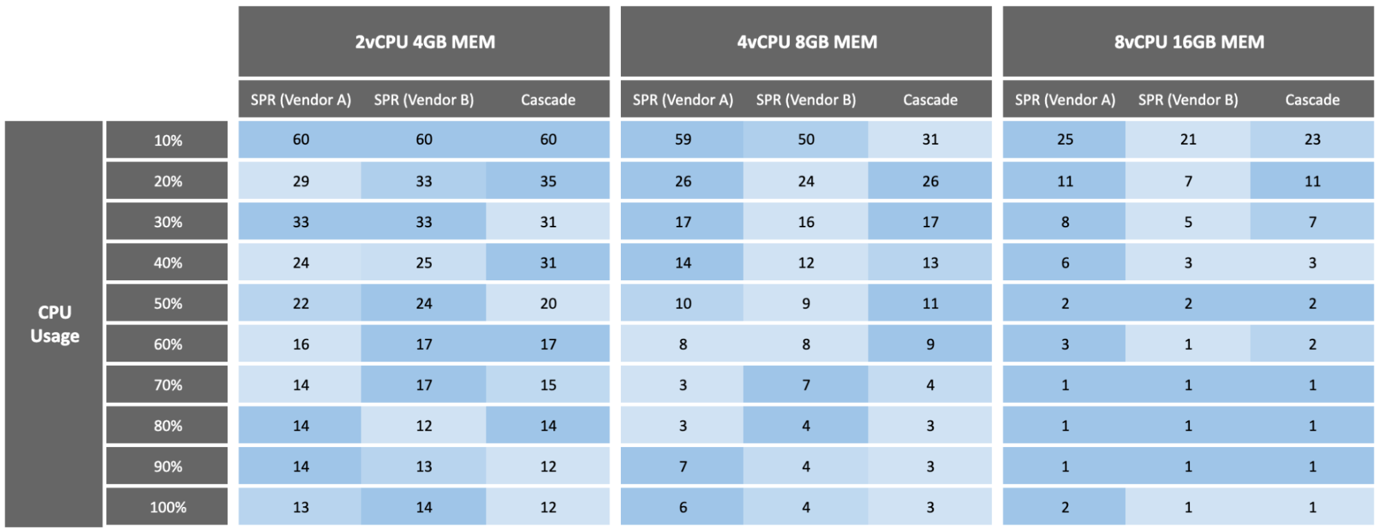
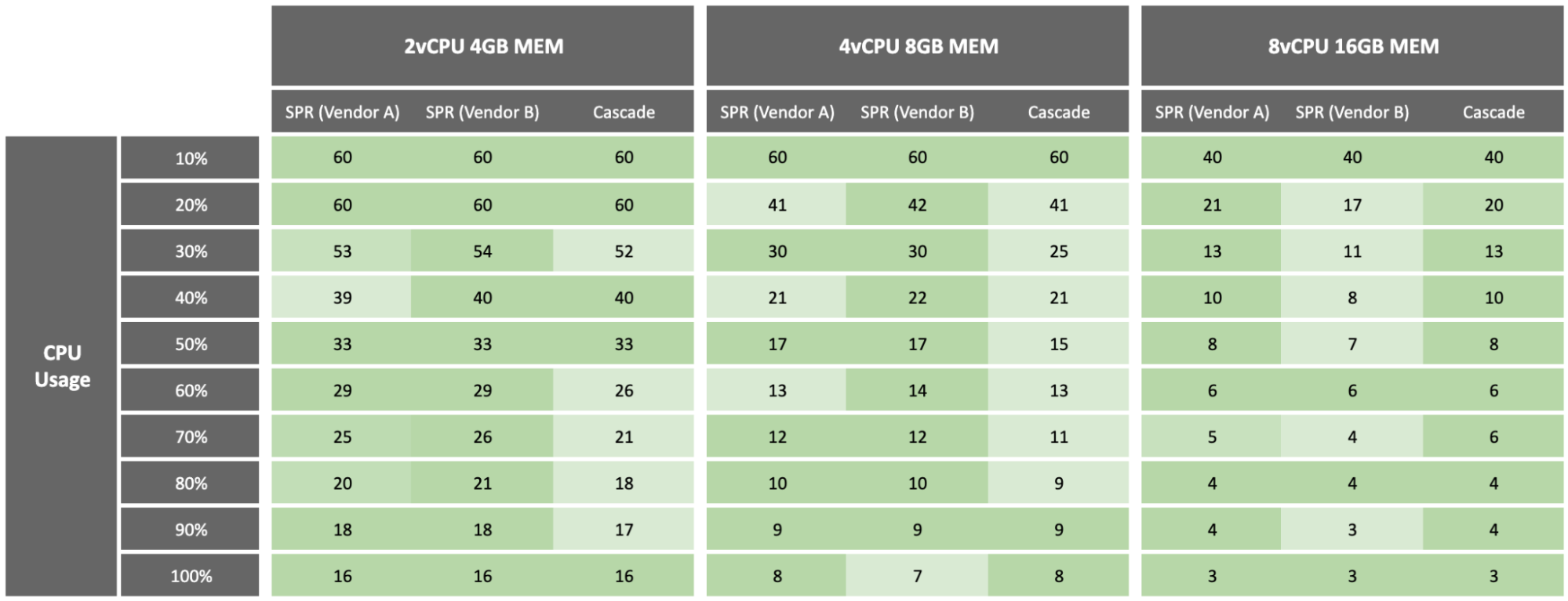
This is the result of translating the maximum number of VMs markers for each CPU performance degradation section from the graph previously introduced, ‘3. Changes in CPU performance of VMs as the number of VMs increases’, to the table.

For each of the 0 - 10%, 10 - 20%, and 20 - 30% sections of the CPU performance degradation for VMs, this table represents the maximum number of VMs that can be accommodated for each PM specification, flavor of VM, and CPU usage of the VM, which can be viewed as the optimal VM density from a CPU perspective.

For each VM CPU usage and VM flavor case, the maximum, median, and minimum values by PM spec are colored differently (darker means more VMs can be accommodated).

This gives an idea of the maximum number of VMs that can be accommodated per PM, assuming some VM CPU degradation can be tolerated.

2) Optimal VM density considering actual operating environment

Based on these results, it is possible to design how many VMs to accommodate per PM in an actual operating environment, knowing the CPU specs of the PM, the flavor of the VMs, and the CPU usage of the VMs.

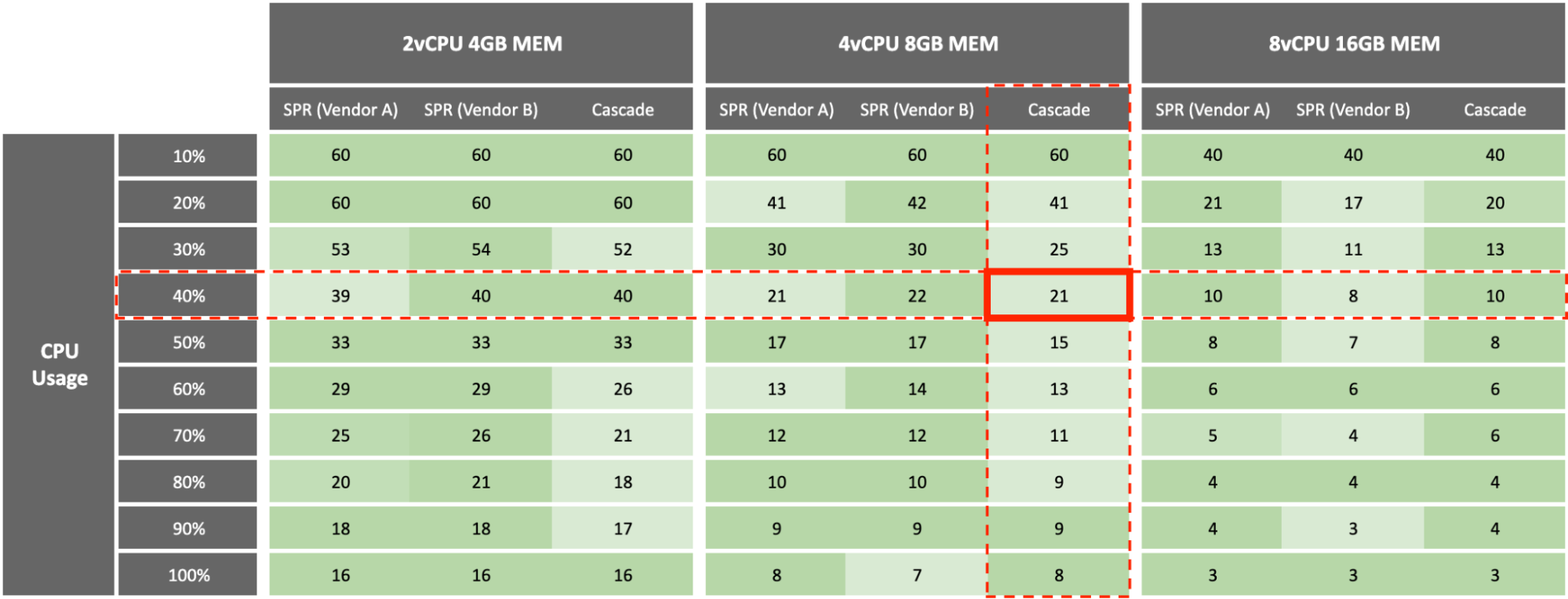
For example, in an environment where VMs of 4 vCPU 8GB MEM flavor are running on a PM with Cascade Silver 4214 @ 2.20GHz CPU specification, assuming that the average CPU usage of the VMs is 40% and the performance degradation of the VMs can be tolerated up to 20%, 21 VMs per PM might be considered.

It’s important to note that this test was conducted from a CPU perspective only, so the results are based on the assumption that PM’s memory and disk specs are sufficient.

6. Ending

In this article, I introduced how to perform VM density testing from a CPU perspective for efficient VMWare infrastructure operations and the results.

In reality, the optimal VM density depends on many system components beyond the CPU, such as memory and disk, and there are many situational variables, such as the needs of the operating environment and services, so the only way to find the optimal value is to actually operate the infrastructure.

Furthermore, the CPU specs of PMs, flavors of VMs, and benchmark programs used in this test are very limited compared to actual environments. Also, in actual operating environments, there are many other practical factors to consider, such as ensuring that there are some idle resources to cope with load spikes, so the optimal VM density values derived from this test are not very meaningful.

However, I think it is meaningful enough to provide insight into the ‘how?’, ‘how much?’, and ‘why?’ of the obvious but vague fact that ‘the performance of VMs decreases as the number of VMs increases because the resources of PMs are limited’. Furthermore, if the VM density test method introduced in this article is applied to memory and disk, not just CPU, and tested under various conditions, more meaningful VM density can be derived.

I hope this has been helpful to you.

Thanks for reading.

---

이 글은 < 효율적인 VMWare 인프라 운영을 위한 최적의 VM 집적도 테스트 >를 영어로 작성한 문서입니다.

다른 번역본 보기:

🇰🇷 한국어: https://tech.kakao.com/posts/634

🇯🇵 日本語: https://tech.kakao.com/posts/637

🇺🇸🇬🇧 English: https://tech.kakao.com/posts/638